Chemometrics & Statistics
12. Experimental Design 2Design of Experiment (DoE)
Initial Thoughts
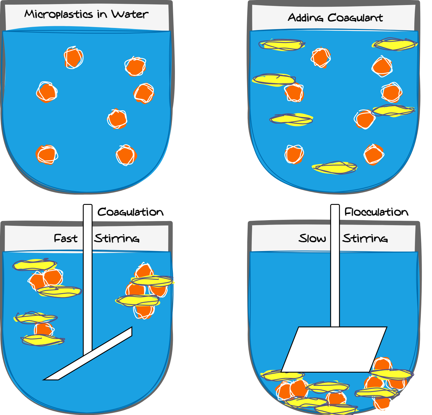
Coagulation process to remove microplastics from water
Factors: Coagulant dosage, pH, stirring speed
Response: Removal efficiency
(% microplastics)
How do process parameters affect microplastic removal efficiency?
Experimental Design: General Info
Experimental Design: A structured approach to planning experiments
Goal: Maximize information while minimizing resources
Focus: Identify key factors and their interactions
Key Benefits:
Improves efficiency and reliability of results
Provides insights into cause-and-effect relationships
Two main Tasks in Experimental Design
1: Method optimization
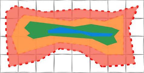
Focus: Identify the best combination of factors (dynamically exploring design space)
Goal: Maximize performance (e.g., sensitivity, efficiency)
Example: Optimizing pH, temperature, and time for a chemical reaction

2: Determination of effects
Focus: Quantify the impact of individual factors and their interactions (statically exploring design space)
Goal: Understand cause-and-effect relationships
Example: Assessing how pH, stirring speed, and dosage influence pollutant removal
Introduction to Design of Experiments (DoE)
What is DoE?
A systematic approach to plan, conduct, and analyze experiments to understand how multiple factors (e.g., water pH, pollutant concentration) affect key outcomes (e.g., degradation efficiency).
Goals of DoE
Characterize relationships between factors and the response to understand their influence on system behavior.
Develop a mathematical model that enables interpolation across the chemical space for predictive analysis.
Capture interactions between factors to identify combined effects on the response.
Key Elements of Experimental Design
Core Components of DoE
Factors: Controlled variables such as pollutant type, pH, or catalyst concentration.
Levels: Specific values, e.g., pollutant concentrations of 10, 50, and 100 mg/L.
Response: Measurable outcomes like pollutant degradation (%) or toxicity reduction.
Why Structure Matters
A structured design helps uncover relationships like how pH influences heavy metal precipitation.
Advantages of Design of Experiments
Efficient Experimentation
DoE minimizes tests needed to determine the optimal dosage of coagulants in water treatment.
Identifies Key Insights
Reveals how interactions between pollutant types and catalysts affect degradation rates.
Improves Process Understanding
Optimizes processes like advanced oxidation or nutrient recovery from wastewater.
Types of Experimental Designs
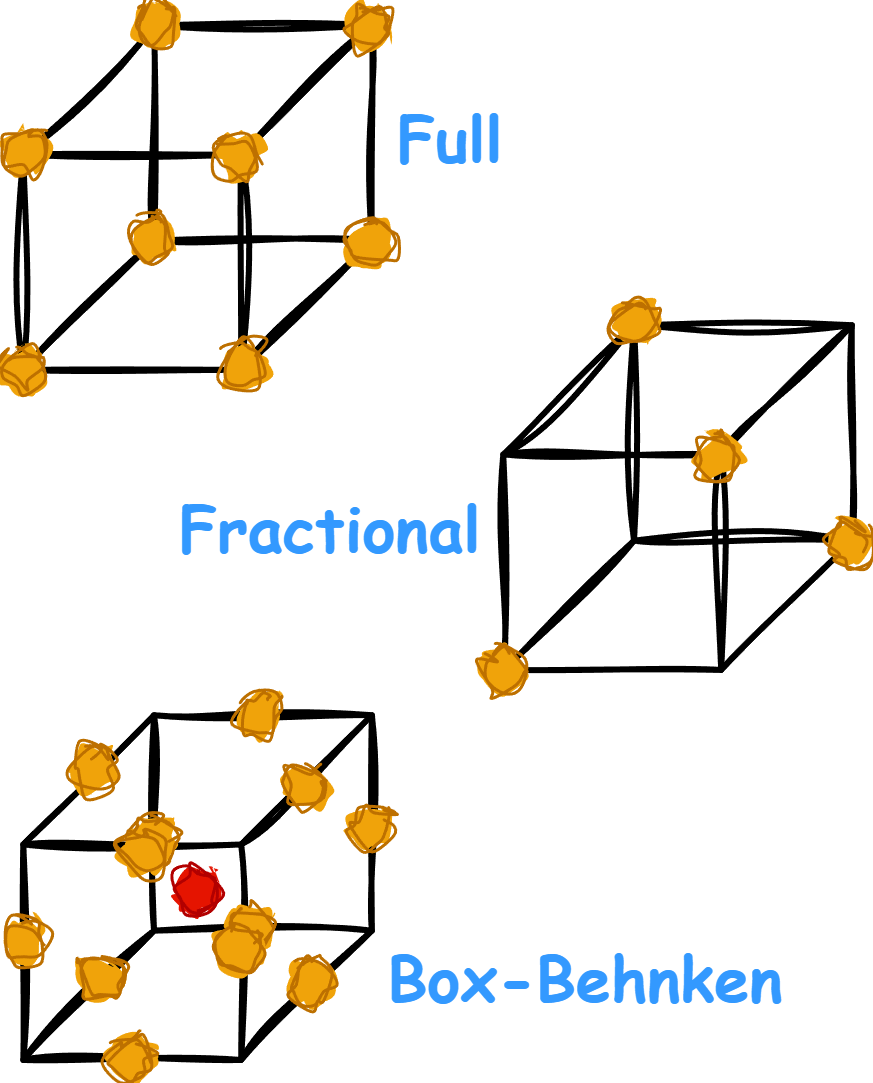
Full Factorial Design
Explores all combinations of factors, e.g., pH, temperature, and pollutant type, providing comprehensive insights.
Fractional Factorial Design
Tests a subset of combinations to reduce effort, e.g., identifying key factors in pesticide degradation.
Box-Behnken Design (BBD)
Efficiently explores factor interactions using midpoints of edges and the center of the design space, avoiding extreme conditions.
Example: Full Factorial Design for Pollutant Removal
Objective
Investigate how temperature and pH influence pollutant removal efficiency in water samples.
Factors and Levels
Factor 1: Temperature → Levels: -1 (Low, 20°C), +1 (High, 40°C)
Factor 2: pH → Levels: -1 (Low, pH 5), +1 (High, pH 9)
Design Type
Full factorial design with 2 levels per factor (2 × 2 = 4 experiments).
Step 1: Creating the Design Matrix
Design Matrix
All combinations of factors and levels (-1, +1) form the matrix.
| Run | Temperature (X₁) | pH (X₂) | Removal Efficiency (Y) |
|---|---|---|---|
| 1 | -1 | -1 | 70 |
| 2 | -1 | +1 | 75 |
| 3 | +1 | -1 | 85 |
| 4 | +1 | +1 | 90 |
Design Matrix (for Regression)
Every factor \(X_i\) is a column in the design matrix, with each row representing a run.
In additon, the very first column is a column of 1s, representing the intercept term.
Intercept can be interpreted as the part of the response that is not explained by the factors. \[ X = \begin{bmatrix} +1 & -1 & -1 \\ +1 & -1 & +1 \\ +1 & +1 & -1 \\ +1 & +1 & +1 \end{bmatrix} \]
Step 2: Regression Analysis
Fitting the Model
Using the data:
Run 1: Y = 70 Run 2: Y = 75 Run 3: Y = 85 Run 4: Y = 90
Estimated Coefficients
β₀: Average response (intercept)
β₁: Effect of temperature on removal efficiency
β₂: Effect of pH on removal efficiency
Example Result
Y = 80 + 7.5X₁ + 2.5X₂
Regression Model
Fit a linear regression model:
Y = β₀ + β₁X₁ + β₂X₂
Y: Removal efficiency (%) X₁: Temperature (-1, +1) X₂: pH (-1, +1)
Apply the Regression
Calculate the coefficients \(\beta_0, \beta_1, \beta_2\) using the design matrix \(X\) and the response vector \(Y\). \[ \begin{bmatrix} \beta_0 \\ \beta_1 \\ \beta_2 \end{bmatrix} = (X^T X)^{-1} X^T Y \]
Step 3: Interpreting Results
Insights from Coefficients
β₁ (7.5): Higher temperature significantly improves removal efficiency.
β₂ (2.5): Higher pH has a smaller positive effect.
Predictions
Predict removal efficiency for any combination of temperature and pH using the regression equation.
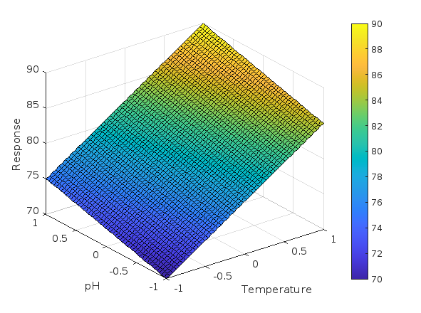
Visualization
Create 2D or 3D plots to illustrate the effects of temperature and pH on removal efficiency.
Step 4: Testing Significance of Coefficients
Hypothesis Testing
For each coefficient (β₁, β₂):
- Null hypothesis (H₀): The coefficient is not significant (β = 0).
- Alternative hypothesis (H₁): The coefficient is significant (β ≠ 0).
t-Test for Significance
Use the formula for the t-statistic:
t = β / SE(β)
Where SE(β) is the standard error of the coefficient.
Decision Rule
Compare the calculated t-value to the critical t-value from the t-distribution table at a chosen significance level (e.g., α = 0.05).
If |t| > critical value, the coefficient is significant.
Example Results
t₁ (β₁ for temperature): Significant (p < 0.05).
t₂ (β₂ for pH): Not significant (p > 0.05).
Step 5: Adjusting Coefficients to Actual Units
Understanding Coefficients
Regression coefficients in coded levels (\([-1, 1]\)) describe the change in response when the factor changes by the full range (\(+2\) units in coded space).
Converting to Real Units
The effect of a factor in real units is calculated by dividing the total response change by the real range of the factor.
Response Change per Real Unit = 2 × β (coded) / Real Range
Example: Temperature
β₁ (coded): 7.5
Real Range: 20°C
Total response change over full range: \( 2 × 7.5 = 15 \)
Change per °C: \( 15 / 20 = 0.75 \) response units per °C
Final Model Interpretation
The temperature coefficient (\( \beta_1 \)) means that for every 1°C increase, the response increases by 0.75 units.
For pH or other factors, use the same formula to adjust the coefficient to the real range.
Determining the Number of Experiments in Full Factorial Designs
Number of Experiments
In a full factorial design, the total number of experiments (\(N\)) depends on the number of factors (\(k\)) and the levels per factor (\(L\)).
Formula
\( N = L^k \)
Where: \(L\): Number of levels per factor (e.g., 2 for \([-1, +1]\)) \(k\): Number of factors
Example
For \(k = 3\) factors (\(X_1, X_2, X_3\)) and \(L = 2\) levels (\([-1, +1]\)):
\( N = 2^3 = 8 \) experiments
Key Insight
The number of experiments grows exponentially with the number of factors. For \(k = 5\) factors and \(L = 2\): \( N = 2^5 = 32 \).
Experiment Count Examples
| Number of Factors (\(k\)) | Experiments (\(N = 2^k\)) |
|---|---|
| 2 | 4 |
| 3 | 8 |
| 4 | 16 |
| 5 | 32 |
Number of Experiments vs. Degrees of Freedom
Degrees of Freedom (df) in Full Factorial Designs
The degrees of freedom (\(df\)) are calculated as:
df = N - p - 1
Where: \(-\) \(N\): Number of experiments \(-\) \(p\): Number of coefficients (factors or interactions) \(-\) \(1\): For the intercept
Model Scenarios
Main Effects Model: Only main factors are included (\(p = k\)).
Main Effects + Pairwise Interactions: Includes main factors and pairwise interactions (\(p = k + \frac{k(k-1)}{2}\)).
Key Insight
The model requires \(df \geq 0\) to estimate coefficients and fit the data. Pairwise interactions significantly increase \(p\), reducing \(df\).
Comparison Table
| Number of Factors (\(k\)) | Experiments (\(N = 2^k\)) | df (Main Effects) | df (Main + Pairwise Interactions) |
|---|---|---|---|
| 2 | 4 | 1 (4 - 2 - 1) |
0 (4 - 3 - 1) |
| 3 | 8 | 4 (8 - 3 - 1) |
1 (8 - 6 - 1) |
| 4 | 16 | 11 (16 - 4 - 1) |
5 (16 - 10 - 1) |
| 5 | 32 | 26 (32 - 5 - 1) |
16 (32 - 15 - 1) |
Understanding Interactions in Experimental Design
What is an Interaction?
An interaction occurs when the effect of one factor on the response depends on the level of another factor.
Interactions highlight synergies or conflicts between factors that cannot be explained by their individual effects alone.
Example
Consider two factors:
Temperature
(\(X_1\)) and pH
(\(X_2\)):
Without interaction: \(Y = \beta_0 + \beta_1 X_1 + \beta_2 X_2\).
With interaction: \(Y = \beta_0 + \beta_1 X_1 + \beta_2 X_2 + \beta_{12} X_1 X_2\).
The interaction term (\(\beta_{12} X_1 X_2\)) modifies the response based on the combination of \(X_1\) and \(X_2\).
Impact on the Design Matrix
Adding interactions introduces new columns to the design matrix, representing products of factors.
Design Matrix Comparison
| Experiment | \(X_1\) | \(X_2\) | \(X_1 X_2\) (Interaction) |
|---|---|---|---|
| 1 | -1 | -1 | 1 |
| 2 | -1 | 1 | -1 |
| 3 | 1 | -1 | -1 |
| 4 | 1 | 1 | 1 |
Understanding Quadratic Terms in Experimental Design
What is a Quadratic Term?
A quadratic term models the nonlinear effects of a factor on the response. It represents the curvature of the relationship between a factor and the response.
Quadratic terms allow for the identification of optimal factor levels, where the response is maximized or minimized.
Example
Consider two factors:
Temperature
(\(X_1\)) and pH (\(X_2\)):
Without quadratic terms: \(Y = \beta_0 + \beta_1 X_1 + \beta_2 X_2 + \beta_{12} X_1 X_2\).
With quadratic terms: \(Y = \beta_0 + \beta_1 X_1 + \beta_2 X_2 + \beta_{12} X_1 X_2 + \beta_{11} X_1^2 + \beta_{22} X_2^2\).
The quadratic terms (\(\beta_{11} X_1^2, \beta_{22} X_2^2\)) allow for curvature in the response.
Impact on the Design Matrix
Adding quadratic terms introduces new columns to the design matrix, representing squared factors.
Design Matrix Comparison
| Experiment | \(X_1\) | \(X_2\) | \(X_1 X_2\) (Interaction) | \(X_1^2\) (Quadratic) | \(X_2^2\) (Quadratic) |
|---|---|---|---|---|---|
| 1 | -1 | -1 | 1 | 1 | 1 |
| 2 | -1 | 1 | -1 | 1 | 1 |
| 3 | 1 | -1 | -1 | 1 | 1 |
| 4 | 1 | 1 | 1 | 1 | 1 |
Is this design plan suitable?
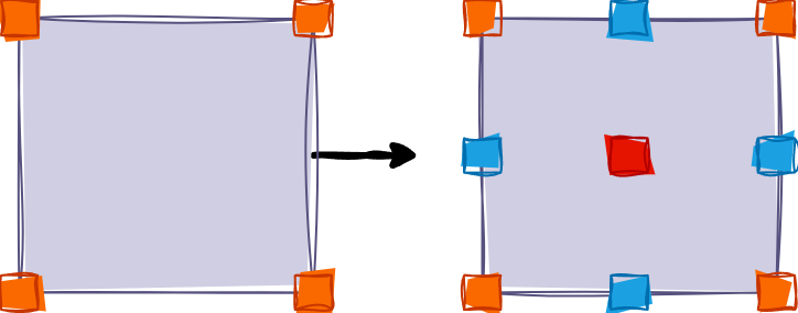
Central and Edge-Center Points in Experimental Design
Why are Additional Points Needed?
To model quadratic terms, additional experiments are required to capture the curvature of the response.
These additional points ensure sufficient information to estimate quadratic effects accurately.
Types of Additional Points
1. Center Points (\(X_1 = 0, X_2 = 0\)): Measure the response at the geometric center of the design space.
2. Edge-Center Points (\(X_1 = 0\) or \(X_2 = 0\)): Measure the response at the midpoint of each factor's range, holding the other factor constant.
Key Insight
Without these points, the curvature of the response cannot be determined, and quadratic terms cannot be estimated reliably.
Updated Design Matrix
| Experiment | \(X_1\) | \(X_2\) | \(X_1 X_2\) (Interaction) | \(X_1^2\) (Quadratic) | \(X_2^2\) (Quadratic) |
|---|---|---|---|---|---|
| 1 | -1 | -1 | 1 | 1 | 1 |
| 2 | -1 | 1 | -1 | 1 | 1 |
| 3 | 1 | -1 | -1 | 1 | 1 |
| 4 | 1 | 1 | 1 | 1 | 1 |
| 5 (Center Point) | 0 | 0 | 0 | 0 | 0 |
| 6 (Edge Center) | 0 | -1 | 0 | 0 | 1 |
| 7 (Edge Center) | 0 | 1 | 0 | 0 | 1 |
| 8 (Edge Center) | -1 | 0 | 0 | 1 | 0 |
| 9 (Edge Center) | 1 | 0 | 0 | 1 | 0 |
Introduction to Fractional Design Plans
Why Use Fractional Designs?
Full factorial designs require exponentially more experiments as the number of factors increases (\(N = 2^k\)).
Fractional designs allow us to study key effects with fewer experiments, saving time and resources.
What is a Fractional Design Plan?
A fractional design tests only a subset (fraction) of the combinations in a full factorial design.
It uses mathematical rules to carefully select combinations that maximize the information gained.
Key Idea
Fractional designs assume that higher-order interactions (e.g., \(X_1 X_2 X_3\)) are negligible, focusing only on main effects and lower-order interactions (e.g., \(X_1 X_2\)).
Benefits of Fractional Designs
Reduces the number of experiments without significantly compromising the quality of insights.
Efficiently identifies main effects and key interactions.
Suitable for initial screening of factors.
Building a Fractional Design Plan
Steps to Create a Fractional Design
1. Start with a full factorial design for a smaller set of factors (e.g., \(X_1, X_2\)).
2. Define additional factors (\(X_3, X_4, \dots\)) as interactions of existing factors.
3. Construct the design matrix by combining these relationships.
Example: Fractional \(2^{3-1}\) Design
\(k = 3\) factors (\(X_1, X_2, X_3\)).
Full factorial: \(2^3 = 8\) experiments.
Fractional plan: \(2^{3-1} = 4\) experiments.
Define \(X_3 = X_1 X_2\).
Fractional Design Matrix
| Experiment | \(X_1\) | \(X_2\) | \(X_3 = X_1 X_2\) |
|---|---|---|---|
| 1 | -1 | -1 | 1 |
| 2 | -1 | 1 | -1 |
| 3 | 1 | -1 | -1 |
| 4 | 1 | 1 | 1 |

Limitations of Fractional Design Plans
Assumptions of Fractional Designs
Fractional designs assume that higher-order interactions are negligible.
If higher-order interactions are significant, the results can be misleading.
Confounding
In fractional designs, some effects are confounded, meaning they cannot be distinguished from each other (same column pattern).
For example, if \(X_3 = X_1 X_2\), the effect of \(X_3\) is inseparable from the interaction \(X_1 X_2\).
Validation is Required
Fractional designs are suitable for initial screening, but full designs or additional experiments may be needed for confirmation.
Key Challenges
Risk of missing significant higher-order interactions.
Interpretation requires careful consideration of confounding.
Reduced resolution compared to full factorial designs.
| Experiment | \(X_1\) | \(X_2\) | \(X_3\) | \(X_1 X_2\) | \(X_1 X_3\) | \(X_2 X_3\) |
|---|---|---|---|---|---|---|
| 1 | -1 | -1 | -1 | 1 | 1 | 1 |
| 2 | -1 | 1 | 1 | -1 | -1 | 1 |
| 3 | 1 | -1 | 1 | -1 | -1 | -1 |
| 4 | 1 | 1 | -1 | 1 | -1 | -1 |
\(X_3\) is confounded with the interaction term \(X_1 \times X_2\).
\(X_1 X_3\) is a hidden quadratic term (\(X_1^2 \times X_2\)), which is not allowed without center points.
\(X_2 X_3\) is a hidden quadratic term (\(X_1 \times X_2^2\)), which is not allowed without center points.
Introduction to Box-Behnken Designs
What is a Box-Behnken Design?
A Box-Behnken design (BBD) is a response surface methodology (RSM) used for modeling nonlinear relationships between factors and responses.
Unlike full factorial designs, BBDs avoid extreme corner points, reducing the risk of running impractical or unsafe experiments.
Key Features
Includes center points (\(X = 0\)) and edge-center points.
Provides sufficient data to estimate quadratic effects.
Requires fewer experiments than a full factorial design.
When to Use?
Box-Behnken designs are ideal when:
Quadratic effects need to be modeled.
Experiments at extreme conditions (e.g., corners) are undesirable.
Benefits of Box-Behnken Designs
Reduces the number of experiments compared to full factorial designs.
Efficiently models curvature (quadratic effects).
Avoids impractical or unsafe experimental conditions.
Structure of a Box-Behnken Design
How is a Box-Behnken Design Built?
Combines edge-center points and center points in the design space.
Requires a minimum of 3 factors (Box-Behnken is not defined for 2 factors).
For 3 factors (\(X_1, X_2, X_3\)), a Box-Behnken plan consists of 12 edge-center points and 1 center point.
Design Matrix Example: 3 Factors
| Experiment | \(X_1\) | \(X_2\) | \(X_3\) |
|---|---|---|---|
| 1 | -1 | 0 | 1 |
| 2 | 1 | 0 | -1 |
| ... | ... | ... | ... |
| 13 (Center Point) | 0 | 0 | 0 |
Key Insight
The Box-Behnken design carefully balances the placement of points to capture quadratic effects while minimizing the number of experiments.
Visualizing a Box-Behnken Plan
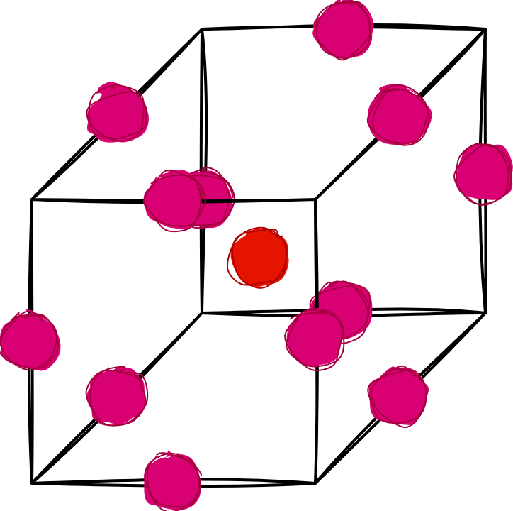
A Box-Behnken design for 3 factors creates a cube with edge-center points and a center point.
Limitations of Box-Behnken Designs
Key Limitations
Not defined for 2 factors; requires at least 3 factors.
Inefficient for large numbers of factors compared to other RSM methods (e.g., Central Composite Designs).
Assumes quadratic effects dominate; may miss higher-order interactions.
Practical Challenges
Limited flexibility for factor ranges; scaling is often required.
Requires careful validation to ensure results are robust.
Example Limitation
With 5 factors, a Box-Behnken design requires significantly more experiments than a fractional factorial design, reducing efficiency.
Key Insight
While Box-Behnken designs are efficient for 3–4 factors, alternative methods may be better for larger systems.
Choosing the Right Experimental Design
Key Considerations
The choice of experimental design depends on:
The number of factors (\(k\)) and their levels (\(L\)).
The type of effects to be studied (main effects, interactions, quadratic terms).
The available resources (time, budget, and experimental feasibility).
Design Overview
| Design Type | When to Use | Key Features |
|---|---|---|
| Full Factorial | Small number of factors (\(k \leq 3\)); all interactions important | Comprehensive insights but resource-intensive |
| Fractional Factorial | Screening for main effects when \(k \geq 4\) | Fewer experiments with confounding of higher-order interactions |
| Box-Behnken | Curvature modeling; \(k = 3\) to \(5\) | No corner points; robust for quadratic effects |
| Central Composite | Curvature modeling; \(k \geq 5\) | Includes axial points; flexible for large ranges |
| ... | ... | ... |
Model Functions for Experimental Designs
Full Factorial
Includes main effects and all interactions:
\( Y = \beta_0 + \beta_1 X_1 + \beta_2 X_2 + \beta_3 X_3 + \beta_{12} X_1 X_2 + \beta_{13} X_1 X_3 + \beta_{23} X_2 X_3 + \beta_{123} X_1 X_2 X_3 \)
Fractional Factorial
Includes only main effects and selected interactions (e.g., confounded terms):
\( Y = \beta_0 + \beta_1 X_1 + \beta_2 X_2 + \beta_{12} X_1
X_2 \)
where \(X_3 = X_1 X_2\)
Box-Behnken
Captures quadratic effects without corner points:
\( Y = \beta_0 + \beta_1 X_1 + \beta_2 X_2 + \beta_3 X_3 + \beta_{12} X_1 X_2 + \beta_{13} X_1 X_3 + \beta_{23} X_2 X_3 + \beta_{11} X_1^2 + \beta_{22} X_2^2 + \beta_{33} X_3^2 \)
Comparison of Models
Full Factorial: Captures all effects but resource-intensive.
Fractional Factorial: Simplified model, ideal for screening.
Box-Behnken: Focuses on quadratic effects, avoids extremes.
Seminar: Optimizing a Water Treatment Process
Backstory
A water treatment facility is seeking to optimize its process for removing pollutants. The response variable of interest is the removal efficiency (%) .
Two factors have been identified as critical to the process:
Temperature (\(X_1\)) : Range \(20^\circ\text{C}\) to \(60^\circ\text{C}\)
pH (\(X_2\)) : Range 6 to 8
Objective
To better understand the influence of these factors, you need to design and execute an experimental plan.
The goal is to identify the factor levels that maximize removal efficiency.
Key Questions
What type of experimental design should you use?
How many experiments are necessary to capture the relevant effects?
Which effects (e.g., main effects, interactions, quadratic effects) should be included in the model?
Your Task
Develop a design plan to investigate the effects of temperature and pH on pollutant removal efficiency.
Create a design matrix that captures the desired effects.
Data