Chemometrics & Statistics
11. Experimental Design 1Downhill-Simplex Optimization
Initial Thoughts
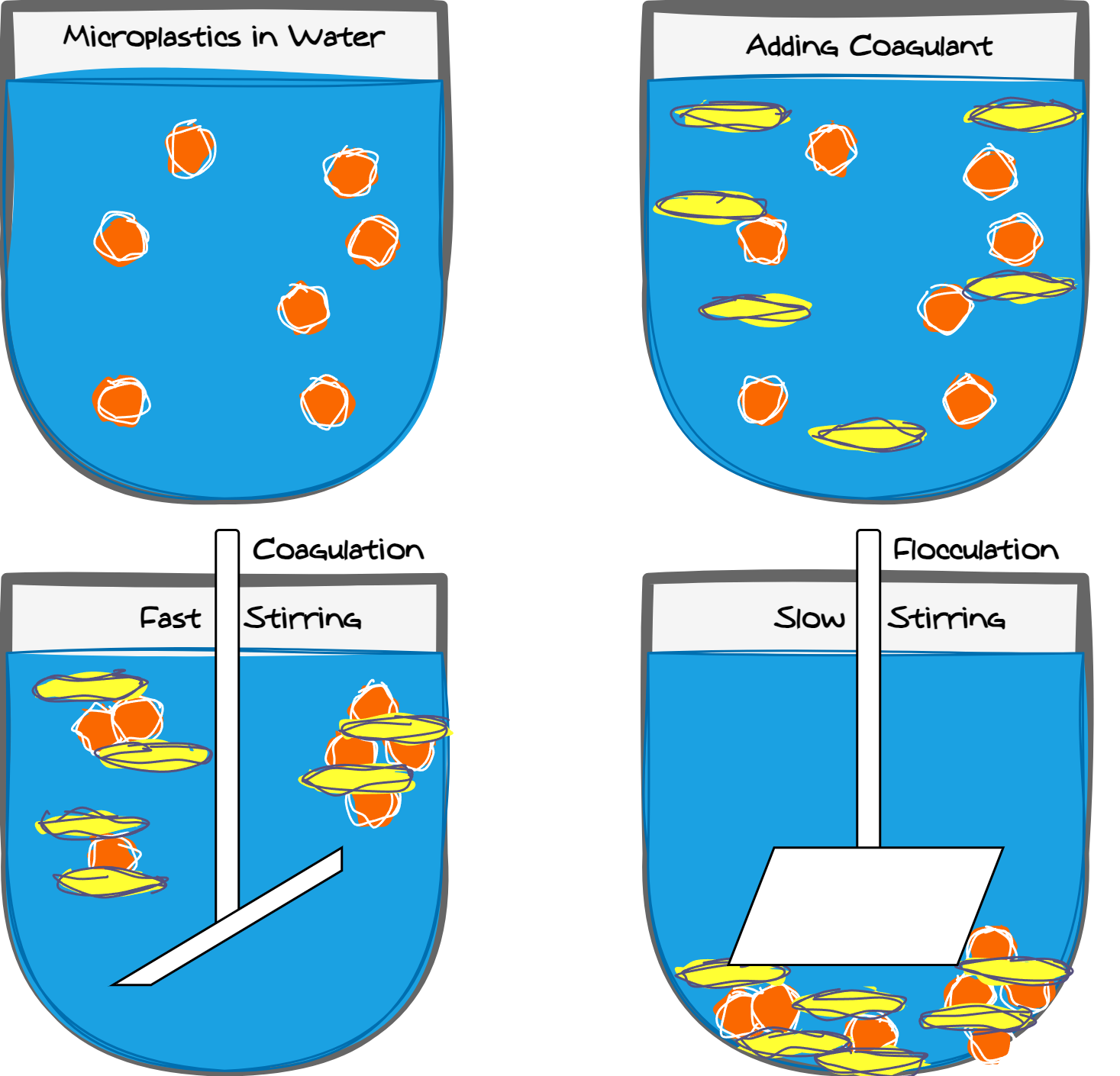
Coagulation process to remove microplastics from water
Factors: Coagulant dosage, pH, stirring speed
Response: Removal efficiency
(% microplastics)
How do process parameters affect microplastic removal efficiency?
Experimental Design: General Info
Experimental Design: A structured approach to planning experiments
Goal: Maximize information while minimizing resources
Focus: Identify key factors and their interactions
Key Benefits:
Improves efficiency and reliability of results
Provides insights into cause-and-effect relationships
Two main Tasks in Experimental Design
1: Method optimization
Focus: Identify the best combination of factors (dynamically exploring design space)
Goal: Maximize performance (e.g., sensitivity, efficiency)
Example: Optimizing pH, temperature, and time for a chemical reaction

2: Determination of effects
Focus: Quantify the impact of individual factors and their interactions (statically exploring design space)
Goal: Understand cause-and-effect relationships
Example: Assessing how pH, stirring speed, and dosage influence pollutant removal
Terms: Factors
Factor: A variable that influences the outcome of an experiment
Also referred to as a parameter
Examples:
pH value in a chemical reaction
Dosage of coagulant in water treatment
Key: Factors can be controlled or adjusted during the experiment
Two types of factors:
Continuous: Can take any value within a range (e.g., pH, temperature)
Categorical: Limited to discrete levels or categories (e.g., type of coagulant: metal salt, polymer)
Definition range: Every factor has a range or set of values it can take
Terms: Response
Response: The dependent variable in an experiment
Also referred to as target or target value
Numeric value: Allows comparison of factor combinations relative to the target
Determined through a model (function) of independent variables (factors)
Choice of model: Crucial for experimental design and depends on the research question
Examples:
Removal efficiency (%) in a coagulation process
Yield of a chemical reaction (e.g., mg product per g reactant)
Limit of detection (LOD) in analytical chemistry
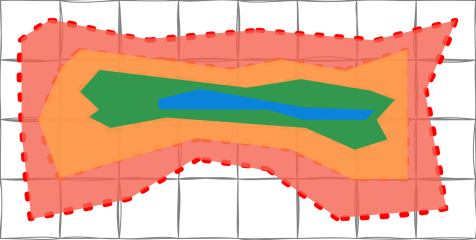
Terms: Experimental Design Space
Experimental Design Space: The range of all possible factor combinations in an experiment
An n+1 dimensional space, where:
n dimensions: Represent the factors (independent variables) as perpendicular axes
1 dimension: Represents the response (dependent variable)
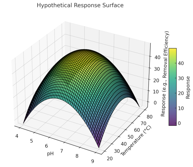
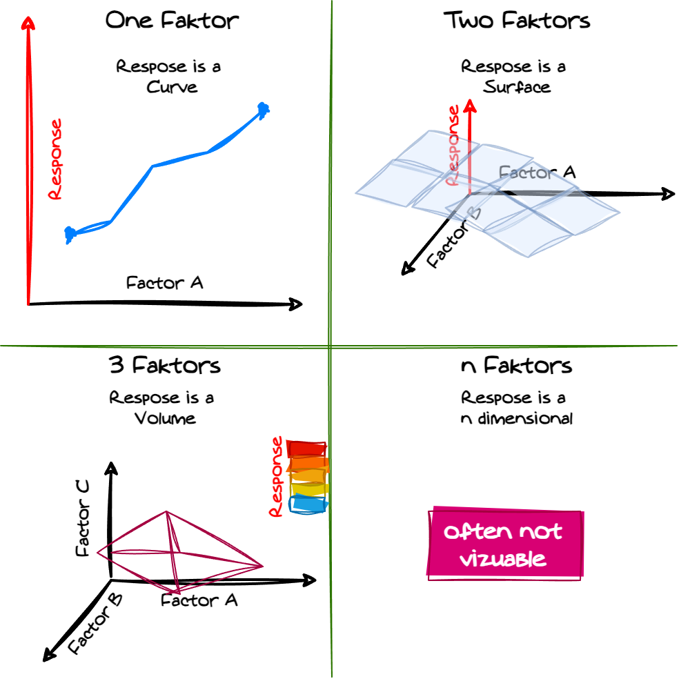
Terms: Dimensionality of the Design Space
For dimensionality of the design space, we have to distinguish between dimensions from factors and the response
The response can be seen as a hyper surface(volume) in the design space
I.e., the response is a function of the factors
This is called the response surface
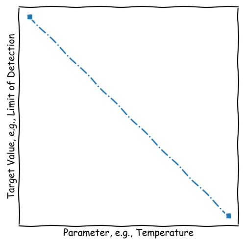
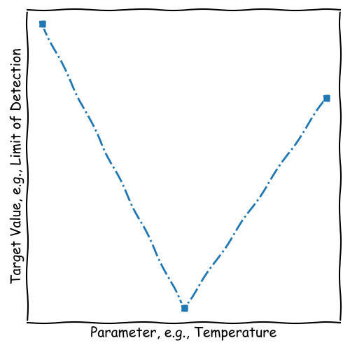
Terms: Resolution of the Design Space
Resolution of the Response Function: Determines the level of detail in the design space
Higher resolution requires more measurement points
For 1 parameter: Resolution increases linearly with the number of measurements
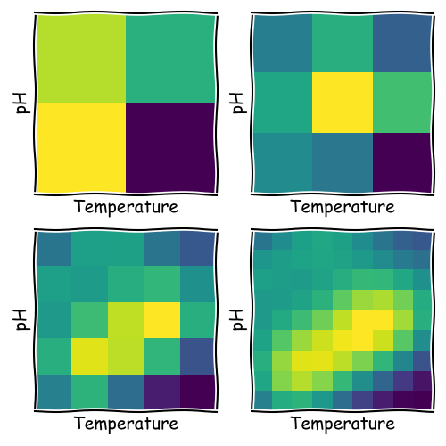
For 2 parameters: Resolution increases quadratically with the number of measurements
Key: Adequate resolution is critical to accurately capture the behavior of the response
Trade-off: High resolution improves detail but increases experimental cost and time
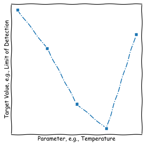
Terms: Resolution of the Design Space
Resolution of the Response Function: Determines the level of detail in the design space
Higher resolution requires more measurement points
For 1 parameter: Resolution increases linearly with the number of measurements
For 2 parameters: Resolution increases quadratically with the number of measurements
Key: Adequate resolution is critical to accurately capture the behavior of the response
Trade-off: High resolution improves detail but increases experimental cost and time
\[ R \propto n^\frac{1}{p} \] where \(R\) is the resolution, \(n\) is the number of measurements, and \(p\) is the number of parameters
I.e., for doubling the resoultion, the number of measurements has to be quadrupled for 2 parameters, cubed for 3 parameters, etc.
Downhill-Simplex Optimization
Downhill Simplex Method: A strategy for response optimization
Focus: Minimize the number of measurement points
Dynamic exploration of the design space
Starts from an initial point and iteratively moves towards the optimal response
Key Features:
Empirical step-by-step response improvement
Well-suited for nonlinear and multidimensional problems
Relies on a geometric approach using an n-simplex (triangle in 2D, tetrahedron in 3D, etc.)
The n-Simplex
n-Simplex: The smallest geometric unit in the design space
Defined by n+1 points in an n-dimensional space
Represents the simplest approximation of the response surface
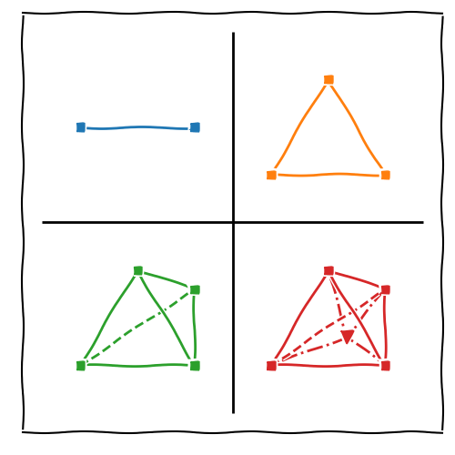
Geometric Interpretation:
for 1 Factor (2D): A line (2 points)
for 2 Factors (3D): A triangle (3 points)
for 3 Factors (4D): A tetrahedron (4 points)
for n Factors: An n-simplex (n+1 points)
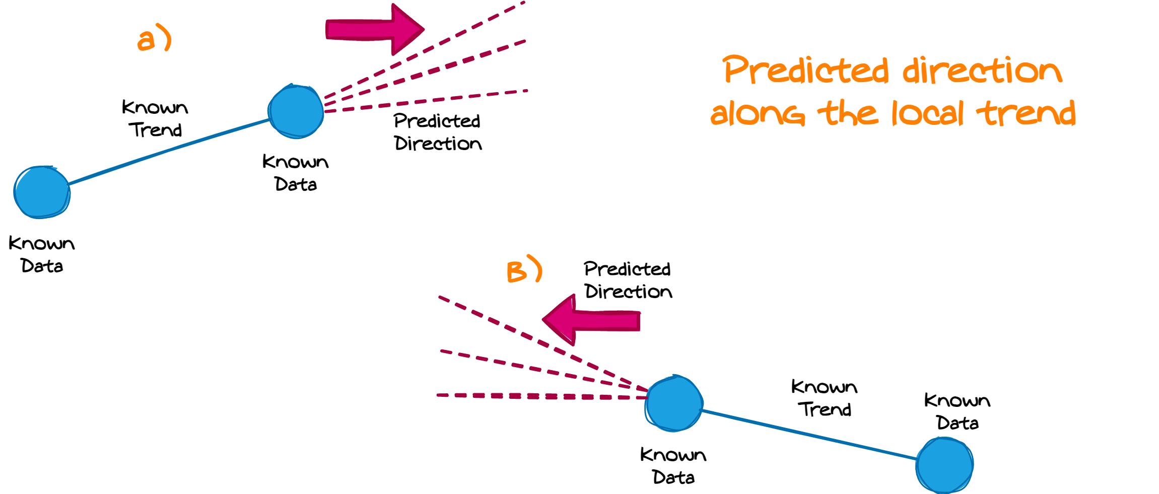
Princple of the Downhill-Simplex Method
We consider the vertices of the n-simplex to estimate local trends of the response surface
We search for improvment algon local trends and reapeat this process until we reach the optimal response
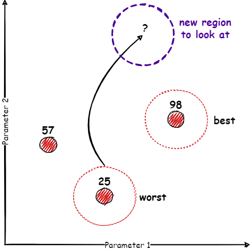
How a Simplex Moves
Principle of the Downhill Simplex:
Iteratively removes the worst point (worst response)
Replaces it with a new point in an unexplored region
Key Step: Reflection
Reflects the worst point across the centroid of the remaining points
Direction of reflection approximates the local gradient
How a Simplex Moves
Principle of the Downhill Simplex:
New point = Reflection Point (R): \[ \mathbf{R} = \mathbf{C} + \alpha (\mathbf{C} - \mathbf{W}) \]
\(\mathbf{C}\): Centroid (mean) of the remaining points
\(\mathbf{W}\): Coordinates of the worst point
\(\alpha\): Reflection coefficient (typically \(\alpha = 1\))
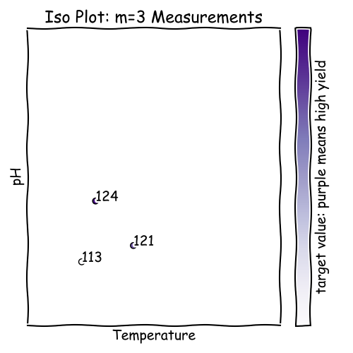
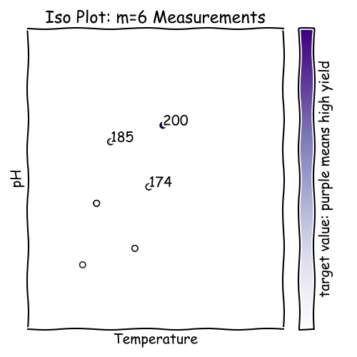
Example
We start with an initial simplex somewhere in the design space
Each point represents a factor combination
In our case we have 2 factors, so the simplex is a triangle
The responses of the points will be evaluated by performing measurements
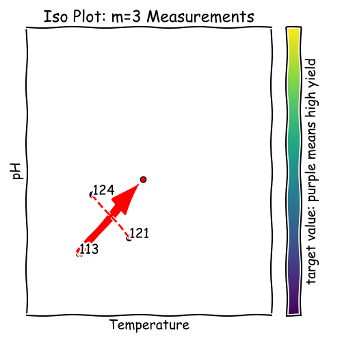
The worst point (113) is reflected across the centroid of the remaining points (124 and 121)
The centroid is calculated dimension-wise, e.g.:
\[C_T=(65+75)/2 = 70\] \[C_{pH}=(4.3 + 4.1)/2 = 4.2\] where {65; 4.3} are the values of the point with the response 124 and {75; 4.1} are the values of the point with the response 121
The reflection point is calculated as:
\[R_T = 70 + 1*(70-62) = 78\] \[R_{pH} = 4.2 + 1*(4.2-4.0) = 4.4\]
The response of the reflection point is measured
The new point has a response of 174
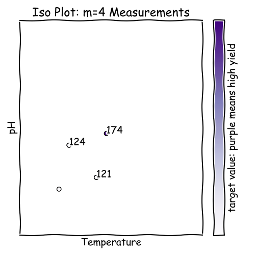
The simplex is updated by replacing the worst point with the reflection point
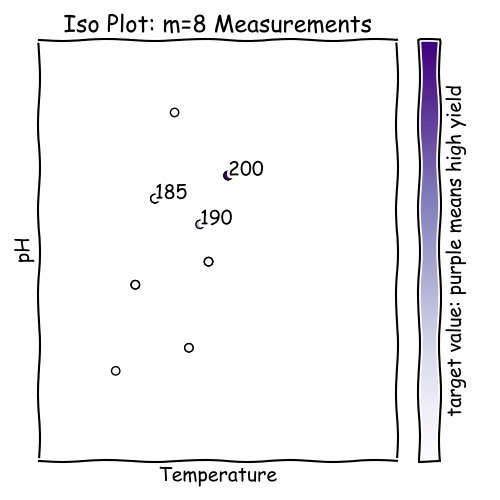
The simplex is then iteratively optimized by repeating the reflection step (now the point 121 is the worst)
The former worst point (121) was reflected across the centroid of the remaining points (124 and 174)
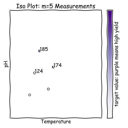
The new point has a response of 185
The simplex is updated by replacing the worst point (121) with the reflection point (185)
The simplex is then iteratively optimized by repeating the reflection step
The former worst point (124) was reflected across the centroid of the remaining points (174 and 185)
The new point has a response of 200
The simplex is updated by replacing the worst point (124) with the reflection point (200)
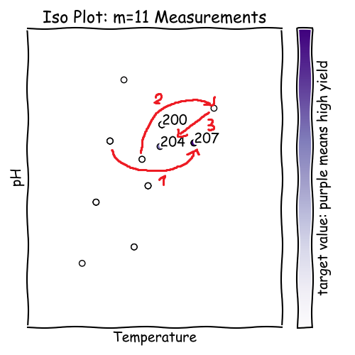
The simplex is then iteratively optimized by repeating the reflection step
The former worst point (174) was reflected across the centroid of the remaining points (185 and 200)
The new point has a response of 183
The simplex is updated by replacing the worst point (174) with the reflection point (183)
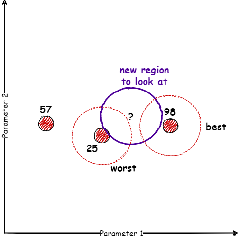
What happens next?

Shrinking / Contracting the Simplex
Shrink: Reducing the simplex size when reflection fails
Occurs when the reflected point is still the worst point
Purpose: Reduce the step size and explore the region more cautiously
Mathematical Step:
New point = Shrink Point (S):
\[
\mathbf{S} = \mathbf{C} + \beta (\mathbf{C} - \mathbf{W})
\]
where \(\beta\) is the shrink coefficient
(typically \(\beta = 0.5\)), \(\mathbf{W}\) is the worst
point
and \(\mathbf{C}\) is the centroid of the remaining points
Goal: Focus exploration on a smaller region
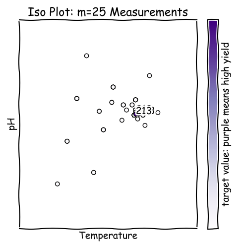
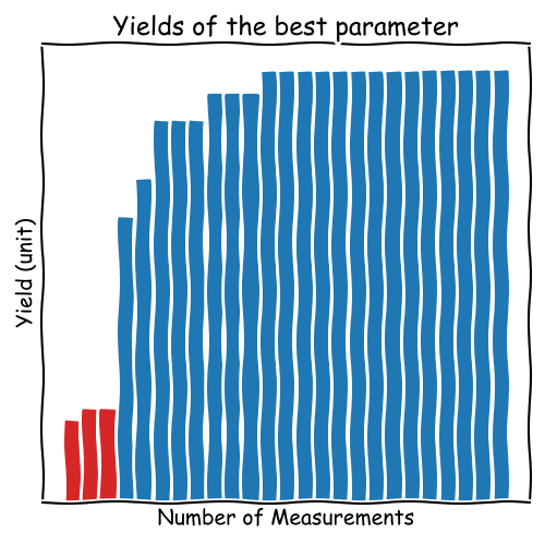
Example: Response Overview
Response Function Across Optimization Steps:
Initial simplex: Individual responses (red bars)
Subsequent steps: Best response per simplex (blue bars)
Rapid improvement followed by saturation
Stopping Criterion:
Occurs when further improvement is negligible
Response convergence: Minimal change in best response (e.g., < 1%)
Simplex size: Simplex shrinks below a predefined threshold
Iteration limit: Maximum number of steps reached (e.g., 25)
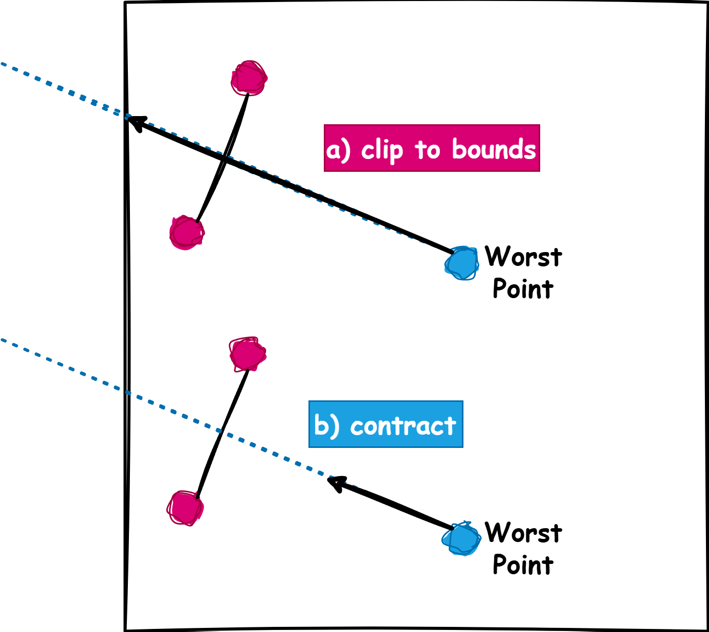
Out of bounds
What to do if the new point leaves the design space?
A new point can fall outside the defined boundaries of the design space
Approaches to handle this:
a) Clip the point: Restrict the new point to the nearest boundary of the design space
b) Modify the reflection or contraction step: Adjust the reflection or shrink coefficient to ensure the point stays within bounds
Example:
If the pH range is 4–9 and a new point suggests pH = 9.5, adjust the point to pH = 9
Alternatively, scale the reflection step to bring the point back within bounds (e.g., \(\alpha = -0.5\))
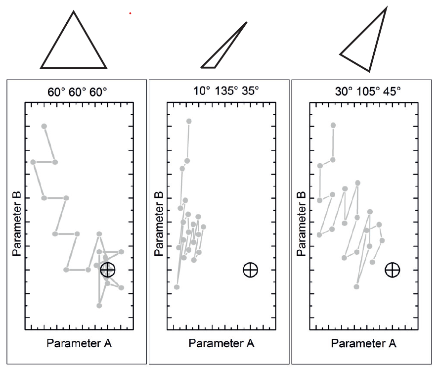
The drunken simplex
Simplex Movement: A "Tumbling" Path to the Optimum
The Simplex does not move directly toward the optimum
Instead, it "tumbles," exploring the response surface dynamically
Reason for Tumbling:
Simplex geometry defines the movement freedom
An irregular Simplex may cause inefficient or erratic motion
Optimal Geometry:
A regular (equilateral) Simplex ensures balanced exploration
Maintains equal "weight" across all dimensions
Goal: Keep the Simplex as regular as possible during optimization
Initial Simplex matters
Importance of the Initial Simplex:
The simplex should be of suitable size, orientation, and shape
Shape: Regular (equilateral)
Size: edge should be like 10% of the design space
avoid edges parallel to the axes
The initial simplex should be placed in a promising region of the design space.
How to create an initial n-simplex
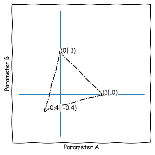
To construct a regular n-simplex we need to find n+1 vertices of n dimensions. E.g., for 2 factors (2D) we need 3 points that form a regular triangle.
Regular means that all edges have the same length and all angles are equal
For a starting, we can use the axes vectors for all but one vertex. The last vertex is then calculated using the rule of Pythagoras.
E.g., for a 2D simplex: \[ \mathbf{A} = \begin{pmatrix} 1 \\ 0 \end{pmatrix} \quad \mathbf{B} = \begin{pmatrix} 0 \\ 1 \end{pmatrix} \quad \mathbf{C} = \begin{pmatrix} ? \\ ? \end{pmatrix} \]
How to create an initial n-simplex
To construct a regular n-simplex we need to find n+1 vertices of n dimensions. E.g., for 2 factors (2D) we need 3 points that form a regular triangle.
Regular means that all edges have the same length and all angles are equal
Now we use that all edges have the same length to calculate the last vertex.
E.g., for a 2D simplex: \[ dist(\mathbf{A}, \mathbf{B}) = dist(\mathbf{B}, \mathbf{C}) = dist(\mathbf{C}, \mathbf{A}) \]
I.e., \[ dist(\mathbf{A}, \mathbf{B}) = \sqrt{(x_A - x_B)^2 + (y_A - y_B)^2} = \sqrt{2} \]
How to create an initial n-simplex
To construct a regular n-simplex we need to find n+1 vertices of n dimensions. E.g., for 2 factors (2D) we need 3 points that form a regular triangle.
Regular means that all edges have the same length and all angles are equal
Now we use that all edges have the same length to calculate the last vertex.
I.e., \[ dist(\mathbf{A}, \mathbf{C}) = \sqrt{(1 - x_C)^2 + (0 - y_C)^2} = \sqrt{2} \] \[ dist(\mathbf{B}, \mathbf{C}) = \sqrt{(0 - x_C)^2 + (1 - y_C)^2} = \sqrt{2} \]
How to create an initial n-simplex
To construct a regular n-simplex we need to find n+1 vertices of n dimensions. E.g., for 2 factors (2D) we need 3 points that form a regular triangle.
Regular means that all edges have the same length and all angles are equal
Now we use that all edges have the same length to calculate the last vertex.
I.e., \[ dist(\mathbf{A}, \mathbf{C}) = dist(\mathbf{B}, \mathbf{C}) \]
\[ \sqrt{(1 - x_C)^2 + (0 - y_C)^2} = \sqrt{(0 - x_C)^2 + (1 - y_C)^2} \]
How to create an initial n-simplex
To construct a regular n-simplex we need to find n+1 vertices of n dimensions. E.g., for 2 factors (2D) we need 3 points that form a regular triangle.
Regular means that all edges have the same length and all angles are equal
Now we use that all edges have the same length to calculate the last vertex.
I.e., \[ dist(\mathbf{A}, \mathbf{C}) = dist(\mathbf{B}, \mathbf{C}) \]
\[ (1 - x_C)^2 + (0 - y_C)^2 = (0 - x_C)^2 + (1 - y_C)^2 \]
How to create an initial n-simplex
To construct a regular n-simplex we need to find n+1 vertices of n dimensions. E.g., for 2 factors (2D) we need 3 points that form a regular triangle.
Regular means that all edges have the same length and all angles are equal
Now we use that all edges have the same length to calculate the last vertex.
I.e., \[ dist(\mathbf{A}, \mathbf{C}) = dist(\mathbf{B}, \mathbf{C}) \]
\[ (1 - x_C)^2 - (0 - x_C)^2 = (1 - y_C)^2 - (0 - y_C)^2 \]
How to create an initial n-simplex
To construct a regular n-simplex we need to find n+1 vertices of n dimensions. E.g., for 2 factors (2D) we need 3 points that form a regular triangle.
Regular means that all edges have the same length and all angles are equal
Now we use that all edges have the same length to calculate the last vertex.
I.e., \[ dist(\mathbf{A}, \mathbf{C}) = dist(\mathbf{B}, \mathbf{C}) \]
\[ x_C = y_C \]
How to create an initial n-simplex
To construct a regular n-simplex we need to find n+1 vertices of n dimensions. E.g., for 2 factors (2D) we need 3 points that form a regular triangle.
Regular means that all edges have the same length and all angles are equal
Now we use that all edges have the same length to calculate the last vertex.
I.e., \[ dist(\mathbf{A}, \mathbf{C}) = \sqrt{2} \]
\[ \sqrt{(1 - x_C)^2 + (0 - y_C)^2} = \sqrt{2} \]
How to create an initial n-simplex
To construct a regular n-simplex we need to find n+1 vertices of n dimensions. E.g., for 2 factors (2D) we need 3 points that form a regular triangle.
Regular means that all edges have the same length and all angles are equal
Now we use that all edges have the same length to calculate the last vertex.
I.e., \[ dist(\mathbf{A}, \mathbf{C}) = \sqrt{2} \]
\[ \sqrt{(1 - u)^2 + (0 - u)^2} = \sqrt{2} \] where \(u\) is \(x_C\) and \(y_C\)
How to create an initial n-simplex
To construct a regular n-simplex we need to find n+1 vertices of n dimensions. E.g., for 2 factors (2D) we need 3 points that form a regular triangle.
Regular means that all edges have the same length and all angles are equal
Now we use that all edges have the same length to calculate the last vertex.
I.e., \[ dist(\mathbf{A}, \mathbf{C}) = \sqrt{2} \]
\[ (1 - u)^2 + (0 - u)^2 = 2 \]
How to create an initial n-simplex
To construct a regular n-simplex we need to find n+1 vertices of n dimensions. E.g., for 2 factors (2D) we need 3 points that form a regular triangle.
Regular means that all edges have the same length and all angles are equal
Now we use that all edges have the same length to calculate the last vertex.
I.e., \[ dist(\mathbf{A}, \mathbf{C}) = \sqrt{2} \]
\[ (1 - u)^2 + u^2 - 2 = 0 \]
How to create an initial n-simplex
To construct a regular n-simplex we need to find n+1 vertices of n dimensions. E.g., for 2 factors (2D) we need 3 points that form a regular triangle.
Regular means that all edges have the same length and all angles are equal
Now we use that all edges have the same length to calculate the last vertex.
I.e., \[ dist(\mathbf{A}, \mathbf{C}) = \sqrt{2} \]
\[ 1 - 2u + u^2 + u^2 - 2 = 0 \]
How to create an initial n-simplex
To construct a regular n-simplex we need to find n+1 vertices of n dimensions. E.g., for 2 factors (2D) we need 3 points that form a regular triangle.
Regular means that all edges have the same length and all angles are equal
Now we use that all edges have the same length to calculate the last vertex.
I.e., \[ dist(\mathbf{A}, \mathbf{C}) = \sqrt{2} \]
\[ 2u^2 - 2u - 1 = 0 \]
How to create an initial n-simplex
To construct a regular n-simplex we need to find n+1 vertices of n dimensions. E.g., for 2 factors (2D) we need 3 points that form a regular triangle.
Regular means that all edges have the same length and all angles are equal
Now we use that all edges have the same length to calculate the last vertex.
I.e., \[ dist(\mathbf{A}, \mathbf{C}) = \sqrt{2} \]
\[ u = \frac{2\pm \sqrt{4 - 4(-1*2)}}{4} = \frac{2\pm \sqrt{12}}{4} = \frac{1\pm \sqrt{3}}{2} \]
Scale the initial simplex
The initial simplex should be scaled that it fits into a normalized design
space
(e.g., 0-1)
To achieve this, we perform a two step approach:
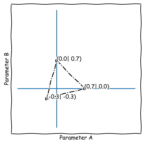
multiply all vertices with the fixed scaling factor of \(1/(\sqrt{2})\) to get the edge length of 1
\[ \mathbf{A_{norm\_edge}} = \mathbf{A} \cdot \frac{1}{\sqrt{2}} \]
Scale the initial simplex
The initial simplex should be scaled that it fits into a normalized design
space
(e.g., 0-1)
To achieve this, we perform a two step approach:
multiply all vertices with the fixed scaling factor of \(1/(\sqrt{2})\) to get the edge length of 1
\[ \mathbf{A_{norm\_edge}} = \mathbf{A} \cdot \frac{1}{\sqrt{2}} \]
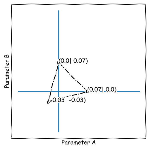
multiply all vertices with the defined scaling factor of e.g. 0.1 or 0.2 to get the desired edge length of 10% or 20% of the design space
\[ \mathbf{A_{scaled}} = \mathbf{A_{norm\_edge}} \cdot 0.1 \]
From normalized simplex to parameters' ranges
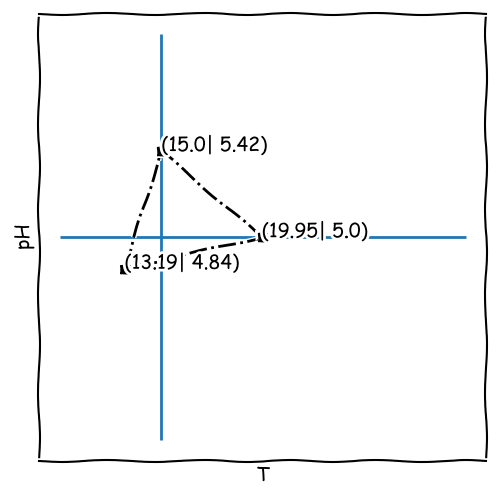
For now, we have a simplex that fits into a normalized design space (e.g., 0-1). However, we want to optimize the parameters within their defined ranges.
To achieve this, we re-scale the simplex to the desired parameter ranges
\[ \mathbf{A_{scaled\_range}} = \mathbf{A_{scaled}} \cdot (\text{max} - \text{min}) + \text{min} \]
for a pH range of 5-8: \[ \mathbf{B_{scaled\_range}} = 0.14 \cdot (8 - 5) + 5 = 5.42 \] (assuming a scaling of 20% in this example)
Rotate the initial simplex
When we construct the initial simplex like described before, it is not aligned with the axes which is already fine.
However, we can rotate the simplex for further improvement using a rotation matrix. E.g., for a 2D simplex:
\[ \begin{pmatrix} x' \\ y' \end{pmatrix} = \begin{pmatrix} \cos(\theta) & -\sin(\theta) \\ \sin(\theta) & \cos(\theta) \end{pmatrix} \begin{pmatrix} x \\ y \end{pmatrix} \]
This step is optional and may not be necessary in all cases.
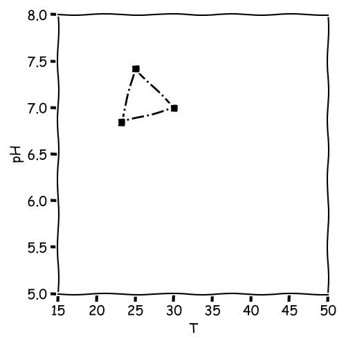
Position the initial simplex
The initial simplex should be placed in a promising region of the design space.
This region should be close to the optimum but not too close to avoid premature convergence.
To achieve this, we use a suitable setting to estimate an offset for the simplex.
\[ \mathbf{A_{offset}} = \mathbf{A_{scaled\_range}} + \text{offset} \]
E.g., for a pH range of 5-8 and an offset of 2: \[ \mathbf{B_{offset}} = 5.42 + 2 = 7.42 \]
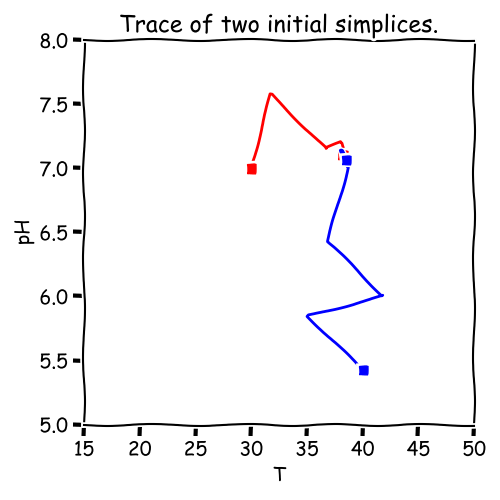
Use mulitple initial Simplexes
In some cases, it might be beneficial to use multiple initial Simplexes to confirm the results.
The reason for this is that the optimum might be local and not global.
Confirmation can be achieved by using different starting points or different scaling factors.
Seminar Materials
Task: Create an initial simplex for the following parameters and their ranges:
pH: 4-6
Temperature T: 38-78°C
Time t: 10-30 min
The simplex should be placed in the center of the design space and cover 5% of the design space (edge length).