10. UncertaintiesLet's assume we have a model that predicts the concentration of a certain analyte in a sample.
As a result, we obtain a concentration of 10.5 mg/L.
What is the problem with this result?
We do not know how reliable this result is.
It makes a huge difference whether the true concentration is...
...10.5 mg/L +/- 0.1 mg/L or...
...10.5 mg/L +/- 5 mg/L.
So the question is: How can we quantify the uncertainty of our result? (Some appraoches you already know.)
When we talk about uncertainties, we can distinguish between different types:
Random uncertainties
Uncertainties caused by natural, unpredictable variations in measurements or samples, even under ideal and consistent conditions. They are characterized by randomness and often follow statistical distributions.
Systematic uncertainties
Uncertainties that consistently shift measurements in a specific direction, arising from identifiable sources like calibration offsets or measurement bias. They are repeatable and predictable but hard to detect without external reference.
Model uncertainties
Uncertainties resulting from limitations in the models used to analyze data or make predictions. These arise from simplifying assumptions, incomplete understanding, or inadequate model complexity.
Key distinctions:
Random uncertainties are inherently variable and can be reduced by averaging multiple measurements.
Systematic uncertainties require calibration or correction to be mitigated, as they affect all measurements consistently.
Model uncertainties are addressed by refining the model, validating its assumptions, or improving the data used for analysis.
However, uncertainties are normal and unavoidable in measurements and analyses, and understanding their nature is crucial for accurate interpretation.
Scenario:
We measure the absorbance (\( E \)) of a solution using the Beer-Lambert law: \[ E = \varepsilon \cdot c \cdot d \] \( \varepsilon \) = molar absorptivity, \( c \) = concentration, \( d \) = path length
For this case:
\( \varepsilon \) and \( d \) are constant and exact.
\( E \) is a random variable due to measurement fluctuations.
Uncertainty of \( E \):
The measurement uncertainty of \( E \) is described by the standard deviation \( \sigma_E \): \[ E \sim N(\mu_E, \sigma_E^2) \]
This uncertainty in \( E \) directly propagates into the calculation of \( c \).
How to improve the uncertainty of \( c \)?
Scenario:
From the Beer-Lambert law, we calculate the concentration: \[ c = \frac{E}{\varepsilon \cdot d} \] where \( \varepsilon \) and \( d \) are constants.
Since \( E \) is a random variable, the uncertainty of \( c \) is calculated using the propagation of uncertainties:
Uncertainty of \( c \):
Using the propagation formula: \[ \sigma_c = \left| \frac{\partial c}{\partial E} \right| \cdot \sigma_E \]
For \( c = \frac{E}{\varepsilon \cdot d} \), the derivative with respect to \( E \) is: \[ \frac{\partial c}{\partial E} = \frac{1}{\varepsilon \cdot d} \]
Substituting: \[ \sigma_c = \frac{\sigma_E}{\varepsilon \cdot d} \]
Key Insight:
The uncertainty in \( c \) is inversely proportional to \( \varepsilon \cdot d \): higher \( \varepsilon \) or \( d \) reduces \( \sigma_c \).
The Problem:
When calculating a new variable (\( z \)) from measured variables (\( x_1, x_2, \dots \)), their uncertainties (\( \sigma_{x_1}, \sigma_{x_2}, \dots \)) affect the uncertainty in \( z \).
The question is: How does \( z \) change when any \( x_i \) changes?
The answer depends on:
The functional relationship between \( z \) and \( x_i \).
The uncertainty (\( \sigma_{x_i} \)) of each variable.
The Solution:
The partial derivative of \( z \) with respect to \( x_i \) tells us how much \( z \) changes when \( x_i \) changes slightly: \[ \frac{\partial z}{\partial x_i} \]
By multiplying this sensitivity by the uncertainty in \( x_i \), we get the contribution of \( x_i \) to the uncertainty in \( z \): \[ \sigma_{z, i} = \left| \frac{\partial z}{\partial x_i} \right| \cdot \sigma_{x_i} \]
Uncertainty in experiments:
Experiments are rarely influenced by a single source of uncertainty.
Uncertainties arise from multiple components, each contributing to the total uncertainty.
These components are often interconnected and must be analyzed to accurately describe the uncertainty of the experiment.
Key sources of uncertainty:
Dependent uncertainties: Shared sources, like calibration or environmental influences, that affect multiple measurements.
Independent uncertainties: Random noise or unrelated systematic effects that act independently.
Goal:
To accurately determine the total uncertainty, we must identify, quantify, and combine all contributing components.
What are dependent uncertainties?
Dependent uncertainties arise from the same source and are fully correlated.
Their effects add in the same direction and reinforce each other.
Examples include calibration errors in multiple sensors using the same faulty standard or environmental factors affecting multiple measurements, such as temperature drift.
How and why do we add dependent uncertainties?
Since dependent uncertainties are fully correlated, their effects are cumulative and must be added directly.
Formula: \( U_{\text{dependent}} = u_1 + u_2 + \dots + u_n \)
This approach reflects the worst-case scenario where all uncertainties push the result in the same direction.
Example:
A balance with a calibration uncertainty of \( \pm 0.1 \, \mathrm{g} \) is used to weigh three samples.
Total mass: \( M_{\text{total}} = m_1 + m_2 + m_3 \)
Total uncertainty: \( U_{\text{total}} = 0.1 + 0.1 + 0.1 = 0.3 \, \mathrm{g} \)
What are independent uncertainties?
Independent uncertainties arise from different, unrelated sources and are not correlated.
Their effects can partially cancel each other out due to randomness.
Examples include random noise in separate measurements or independent biases in unrelated instruments.
How and why do we add independent uncertainties?
Independent uncertainties act as orthogonal components and combine through the quadratic sum.
Formula: \( U_{\text{independent}} = \sqrt{u_1^2 + u_2^2 + \dots + u_n^2} \)
This reflects the combined variability while avoiding overestimation, as random effects may cancel out.
Example:
Three masses are measured independently with the following uncertainties: \[ m_1 = 5.0 \pm 0.1 \, \mathrm{g}, \, m_2 = 10.0 \pm 0.2 \, \mathrm{g}, \, m_3 = 15.0 \pm 0.3 \, \mathrm{g} \]
Total mass: \( M_{\text{total}} = m_1 + m_2 + m_3 = 30.0 \, \mathrm{g} \)
Total uncertainty: \( U_{\text{independent}} = \sqrt{(0.1)^2 + (0.2)^2 + (0.3)^2} \)
The Question:
Why does the total uncertainty seem smaller when using three independent scales compared to using one scale, even if all have the same uncertainty?
Scenario:
Case 1: Three independent scales with uncertainties: \[ u_1 = 0.3 \, \mathrm{g}, \, u_2 = 0.3 \, \mathrm{g}, \, u_3 = 0.3 \, \mathrm{g} \] Total uncertainty: \[ U_{\text{independent}} = \sqrt{(0.3)^2 + (0.3)^2 + (0.3)^2} = 0.52 \, \mathrm{g} \]
Case 2: One scale used three times with a systematic uncertainty of: \[ u = 0.3 \, \mathrm{g} \] Total uncertainty (dependent): \[ U_{\text{dependent}} = 0.3 + 0.3 + 0.3 = 0.9 \, \mathrm{g} \]
Why does this happen?
In independent uncertainties, random errors can partially cancel out due to their uncorrelated nature. This leads to a smaller total uncertainty.
In dependent uncertainties, all errors reinforce each other because they are fully correlated, resulting in a larger total uncertainty.
Key Takeaway:
Independent uncertainties reduce the overall variability due to the statistical nature of random errors, whereas dependent uncertainties model the worst-case scenario of cumulative bias.
What happens when both types are present?
In real systems, uncertainties often include both dependent and independent contributions.
Examples include calibration errors combined with random noise in measurements or systematic environmental influences combined with unrelated biases.
How to combine dependent and independent uncertainties?
Dependent uncertainties are added directly, and independent uncertainties are combined using the quadratic sum.
The two groups are then combined quadratically.
Formula: \[ U_{\text{total}} = \sqrt{U_{\text{dependent}}^2 + U_{\text{independent}}^2} \]
This approach accounts for both cumulative effects and orthogonal contributions.
What is a Round-Robin Test?
A collaborative testing approach where multiple laboratories measure the same sample to evaluate:
Random uncertainties (independent) from individual measurement conditions.
Systematic uncertainties (dependent) caused by shared influences, such as calibration standards or environmental factors.
Why is it used?
To assess the reliability and reproducibility of a method and identify the main sources of uncertainty.
How are uncertainties combined?
Independent uncertainties from each lab are combined quadratically: \[ U_{\text{random}} = \sqrt{\frac{\sum_{i=1}^n (x_i - \bar{x})^2}{n-1}} \]
Systematic uncertainty is determined from the mean bias between the lab results and the reference value: \[ U_{\text{systematic}} = \left| \frac{\sum_{i=1}^n (x_i - x_{\text{ref}})}{n} \right| \]
Total uncertainty combines both contributions: \[ U_{\text{total}} = \sqrt{U_{\text{random}}^2 + U_{\text{systematic}}^2} \]
Scenario:
Three laboratories measure the mass of the same sample:
\( x_1 = 100.2 \, \mathrm{g}, \, x_2 = 99.8 \, \mathrm{g}, \, x_3 = 100.1 \, \mathrm{g} \)
Reference value: \( x_{\text{ref}} = 100.0 \, \mathrm{g} \)
Measurement uncertainties:
\( u_1 = 0.2 \, \mathrm{g}, \, u_2 = 0.3 \, \mathrm{g}, \, u_3 = 0.1 \, \mathrm{g} \)
Step 1: Random uncertainty
Random Uncertainty of lab measurements: \[ U_{\text{random}} = \sqrt{\frac{\sum_{i=1}^3 (x_i - \bar{x})^2}{3-1}} \] \[ U_{\text{random}} = \sqrt{\frac{0.033^2 + 0.233^2 + 0.067^2}{2}} \approx 0.16 \, \mathrm{g} \]
Step 2: Systematic uncertainty
Mean bias relative to reference: \[ U_{\text{systematic}} = \left| \frac{\sum_{i=1}^3 (x_i - x_{\text{ref}})}{3} \right| \] \[ U_{\text{systematic}} = \left| \frac{0.2 - 0.2 + 0.1}{3} \right| = 0.033 \, \mathrm{g} \]
Step 3: Total uncertainty
Combine random and systematic uncertainties: \[ U_{\text{total}} = \sqrt{U_{\text{random}}^2 + U_{\text{systematic}}^2} \] \[ U_{\text{total}} = \sqrt{(0.16)^2 + (0.033)^2} \approx 0.163 \, \mathrm{g} \]
Conclusion:
The propotion of the total uncertainty is due to random errors, while the systematic uncertainty is relatively small. The total uncertainty is 0.163 g should be reported for the mass measurement when applying the Round-Robin validated method.
What is uncertainty propagation?
When calculating a new variable (\( z \)) from measured variables (\( x_1, x_2, \dots \)), the uncertainties in \( x_i \) affect \( z \).
The goal is to estimate the uncertainty of \( z \), denoted \( \sigma_z \), based on the uncertainties of \( x_i \).
How does it work?
If \( z \) is a function of \( x_1, x_2, \dots, x_n \): \[ z = f(x_1, x_2, \dots, x_n) \]
The uncertainty of \( z \) is approximated by: \[ \sigma_z = \sqrt{\sum_{i=1}^n \left( \frac{\partial f}{\partial x_i} \cdot \sigma_{x_i} \right)^2} \]
Each term \( \frac{\partial f}{\partial x_i} \cdot \sigma_{x_i} \) represents the contribution of \( x_i \) to the total uncertainty.
Scenario:
The Beer-Lambert law relates absorbance (\( E \)) to concentration (\( c \)): \[ c = \frac{E}{\varepsilon \cdot d} \]
Uncertainties:
\( \sigma_E = 0.01, \, \sigma_\varepsilon = 0.05, \, \sigma_d = 0.02 \)
Measured values:
\( E = 1.0, \, \varepsilon = 100.0, \, d = 1.0 \, \mathrm{cm} \)
Step 1: Partial derivatives
\[ \frac{\partial c}{\partial E} = \frac{1}{\varepsilon \cdot d}, \quad \frac{\partial c}{\partial \varepsilon} = -\frac{E}{\varepsilon^2 \cdot d}, \quad \frac{\partial c}{\partial d} = -\frac{E}{\varepsilon \cdot d^2} \]
Step 2: Propagate uncertainties
\[ \sigma_c = \sqrt{\left( \frac{\partial c}{\partial E} \cdot \sigma_E \right)^2 + \left( \frac{\partial c}{\partial \varepsilon} \cdot \sigma_\varepsilon \right)^2 + \left( \frac{\partial c}{\partial d} \cdot \sigma_d \right)^2} \]
Step 3: Numerical values
\[ \frac{\partial c}{\partial E} = 0.01, \quad \frac{\partial c}{\partial \varepsilon} = -0.0001, \quad \frac{\partial c}{\partial d} = -0.01 \]
\[ \sigma_c = \sqrt{(0.0001)^2 + (0.000005)^2 + (0.0002)^2} \approx 0.00022 \]
Result:
Concentration \( c = 0.01 \, \mathrm{mol/L} \pm 0.0002 \, \mathrm{mol/L} \)
What are significant figures?
Significant figures reflect the precision of a measurement or calculation. They include all certain digits and the first uncertain digit.
Rules for significant figures:
Non-zero digits are always significant.
Zeros between significant digits are significant.
Leading zeros are not significant.
Trailing zeros in a number with a decimal point are significant.
Examples:
\( 0.0045 \): 2 significant figures (\( 4 \) and \( 5 \)).
\( 450.0 \): 4 significant figures (\( 4, 5, 0, 0 \)).
\( 1500 \): 2 significant figures (\( 1 \) and \( 5 \))
\( 1.5 \times 10^3 \): 2 significant figures (\( 1 \) and \( 5 \)).
\( 1500. \): 4 significant figures (\( 1, 5, 0, 0 \)).
\( 1500.0 \): 5 significant figures (\( 1, 5, 0, 0, 0 \)).
When performing calculations:
For multiplication/division: Result has the same significant figures as the input with the fewest significant figures.
E.g., \( 12.34 \times 3.2 = 39 \) (rounded to 2 significant figures).
For addition/subtraction: Result has the same decimal places as the input with the fewest decimal places.
E.g., \( 123.456 + 0.12 = 123.58 \) (rounded to 2 decimal places).
Why report uncertainties?
Uncertainties communicate the reliability of a measurement and provide a range where the true value is likely to lie.
Common formats:
\( x \pm u \): Value with uncertainty
E.g., \( 12.3 \pm 0.1 \).
Parentheses notation: \( x(u) \): Uncertainty in the last digit(s)
E.g., \( 12.3(1) \) = \( 12.3 \pm 0.1 \).
E.g., \( 12.345(12) \) = \( 12.345 \pm 0.012 \).
Rules for reporting uncertainties:
The uncertainty is usually reported to 1 or 2 significant figures.
The value is rounded to the same decimal place as the uncertainty.
Examples:
Measurement: \( 123.456 \pm 0.12 \):
Reported as \( 123.46 \pm 0.12 \).
Parentheses notation: \( 123.46(12) \).
Errors:
Describe the actual deviation of a discrete result from the true value.
Refer to specific measurements or calculations.
Can be corrected if the source is identified.
Example: A measured value of 22.1 °C has an error of -0.4 °C if the true value is 22.5 °C.
Uncertainties:
Describe the range within which the true value is likely to lie.
Statistical representation of possible deviations.
Account for both random variability and systematic influences.
Example: An uncertainty of ±0.5 °C means the true value is likely between 21.6 °C - 22.6 °C.
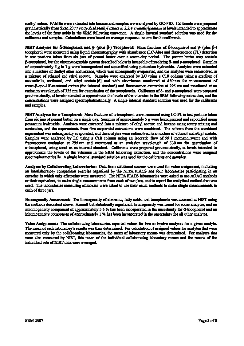
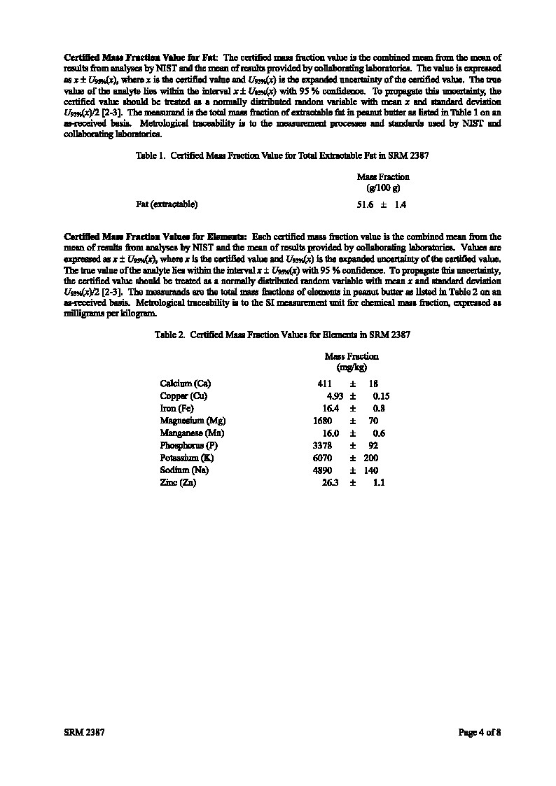
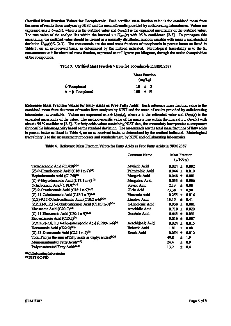
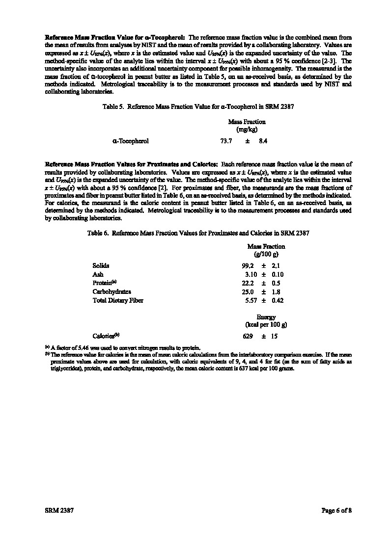
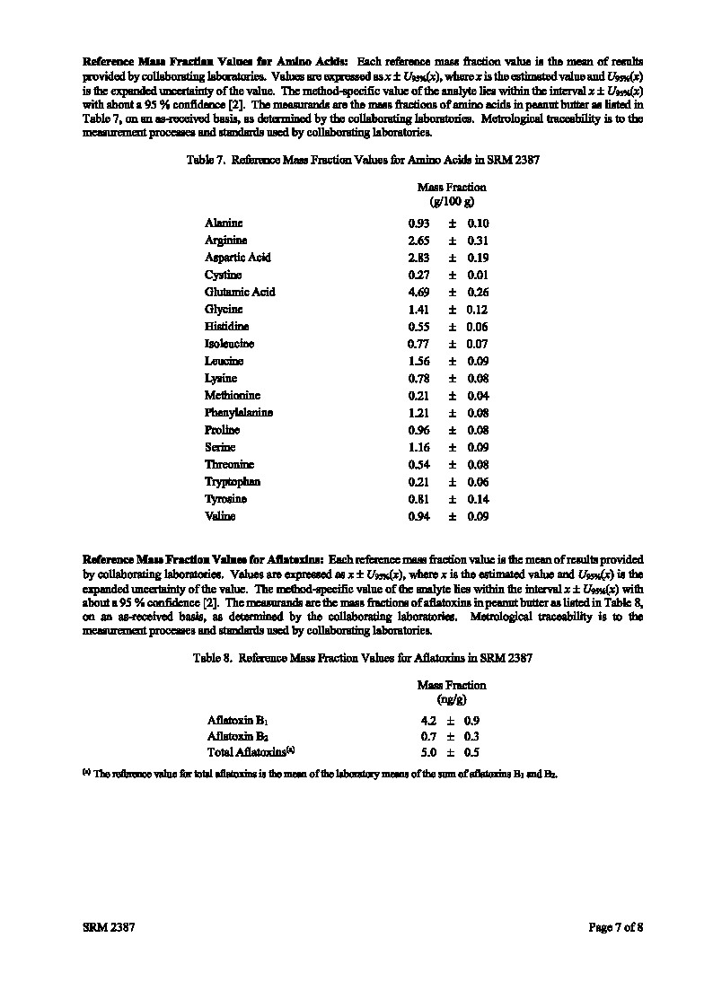
What are SRMs?
Certified materials with well-defined composition or properties, issued by official institutions (e.g., NIST, BAM, etc.).
Used to validate measurement methods and assess measurement errors.
Help ensure traceability to international standards.
Cover a wide range of applications (e.g., chemical composition, physical properties).
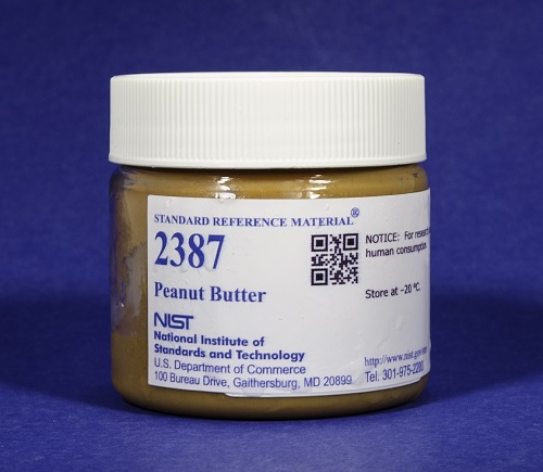
Example: Peanut butter as a standard reference material for food analysis. Do not eat this it costs $1,143.00 per jar.
How is SRM Trueness Defined?
Typically established through inter-laboratory comparisons (e.g., round robin tests).
Certified values are based on consensus results from multiple, independent laboratories.
Measurement uncertainty is rigorously evaluated and reported with the certified value.
Validation includes comparison against primary standards or highly accurate reference methods.
Why correct errors?
Errors cause deviations from the true value, reducing the reliability and accuracy of results.
Correcting errors ensures better data quality, improving confidence in experimental findings.
Reduces the propagation of errors in subsequent calculations or analyses.
How to correct errors:
Identify the source: Understand if errors are due to calibration, environmental influences, measurement procedures, or instrument bias.
Use reference materials: Compare results with certified reference values to detect and correct systematic deviations.
Apply corrections: Adjust results based on known biases or systematic shifts identified during validation.
Verify corrections: Reassess data consistency after correction to ensure the desired accuracy is achieved.
Scenario:
A thermometer is used to measure the temperature of a water bath. The true value, determined using a Standard Reference Material (SRM), is \( 25.00 \, {}^\circ\mathrm{C} \). However, the thermometer consistently reads \( 24.80 \, {}^\circ\mathrm{C} \).
Identified Error: A systematic bias of \( -0.20 \, {}^\circ\mathrm{C} \) in the thermometer's readings.
Correction Calculation:
Measured Value: \( 24.80 \, {}^\circ\mathrm{C} \)
Correction Factor: \( +0.20 \, {}^\circ\mathrm{C} \)
Corrected Value:
\[ T_{\text{corrected}} = T_{\text{measured}} + \text{Correction Factor} \]
Substituting values:
\[ T_{\text{corrected}} = 24.80 + 0.20 = 25.00 \, {}^\circ\mathrm{C} \]
The corrected value matches the true value from the SRM.
Scenario:
A measurement instrument experiences drift over time. A standard sample with a known value of \( 50.00 \, {}^\circ\mathrm{C} \) is periodically measured to monitor the drift.
The following measurements are taken:
At \( t = 0 \): Measured standard = \( 50.00 \, {}^\circ\mathrm{C} \) (no drift)
At \( t = 1 \): Measured standard = \( 50.20 \, {}^\circ\mathrm{C} \) (+0.20 drift)
At \( t = 2 \): Measured standard = \( 50.50 \, {}^\circ\mathrm{C} \) (+0.50 drift)
Correction Calculation:
Measured sample value at \( t = 2 \): \( 47.80 \, {}^\circ\mathrm{C} \)
Measured standard drift at \( t = 2 \): \( +0.50 \, {}^\circ\mathrm{C} \)
Corrected sample value:
\[ T_{\text{corrected}} = T_{\text{measured}} - \text{Drift Correction} \]
Substituting values:
\[ T_{\text{corrected}} = 47.80 - 0.50 = 47.30 \, {}^\circ\mathrm{C} \]
Using the standard sample allows for accurate correction of the time-dependent drift.
Scenario:
In high-frequency drift situations (e.g., isotope measurements), drift corrections are performed using flanking standards.
Two standards with known values are measured before and after the sample to interpolate the correction term.
Example measurements:
Standard 1 (before sample): Measured = \( 1.010 \), True = \( 1.000 \), Drift = \( +0.010 \)
Standard 2 (after sample): Measured = \( 1.015 \), True = \( 1.000 \), Drift = \( +0.015 \)
Sample measurement: Measured = \( 1.008 \)
Correction Calculation:
Step 1: Interpolate drift correction for sample time:
\[ \text{Drift}_{\text{sample}} = \text{Drift}_{\text{before}} + \frac{\text{Drift}_{\text{after}} - \text{Drift}_{\text{before}}}{2} \]
Substituting values:
\[ \text{Drift}_{\text{sample}} = 0.010 + \frac{0.015 - 0.010}{2} = 0.0125 \]
Step 2: Correct the sample value:
\[ \text{Corrected}_{\text{sample}} = \text{Measured}_{\text{sample}} - \text{Drift}_{\text{sample}} \]
Substituting values:
\[ \text{Corrected Sample Value} = 1.008 - 0.0125 = 0.9955 \]
The corrected sample value accurately accounts for high-frequency drift.
What are outliers?
Outliers are data points that deviate significantly from the rest of the dataset. They can:
Indicate errors: Measurement or recording mistakes.
Represent rare but valid events: Anomalies in natural phenomena.
Common outlier tests:
Interquartile Range (IQR): Classifies outliers as points beyond \( 1.5 \times \mathrm{IQR} \) from the first or third quartile.
Outliers:
\( x < Q_1 - 1.5 \times \mathrm{IQR} \) or \( x > Q_3 + 1.5 \times \mathrm{IQR} \)
Where \( \mathrm{IQR} = Q_3 - Q_1 \).
Grubbs' Test: Identifies one outlier at a time in normally distributed data. \[ G = \frac{|x_i - \bar{x}|}{s} \] Where \( G \) is the test statistic, \( x_i \) the suspected outlier, \( \bar{x} \) the mean, and \( s \) the standard deviation.
Critical value (\( G_{\text{crit}} \)): Depends on the sample size \( n \) and confidence level \( \alpha \).
\[
G_{\text{crit}} = \frac{n-1}{\sqrt{n} \cdot \sqrt{n-2 + \frac{t^2}{n-1}}}
\]
Where \( t \) is the critical value of the t-distribution with \( n-2 \) degrees of freedom.
Dixon's Q Test: Useful for small datasets, compares the gap between the outlier and its nearest neighbor to the range of the data.
Critical value (\( Q_{\text{crit}} \)): Depends on sample size and confidence level. Example for \( n = 5, \alpha = 0.05 \): \( Q_{\text{crit}} = 0.71 \).
Dataset:
\( [12, 15, 13, 14, 22] \)
Grubbs' Test:
\[
G = \frac{|22 - 15.2|}{3.6} \approx 1.89
\]
Critical value: \( G_{\text{crit}} = 1.67 \, (\alpha = 0.05, n = 5) \).
Result: \( 22 \) is an outlier (\( G > G_{\text{crit}} \)).
Dixon's Q Test:
\[
Q = \frac{|22 - 15|}{22 - 12} = \frac{7}{10} = 0.7
\]
Critical value: \( Q_{\text{crit}} = 0.71 \, (\alpha = 0.05, n = 5) \).
Result: \( 22 \) is not an outlier (\( Q < Q_{\text{crit}} \)).
After removing the outlier:
New dataset: \( [12, 15, 13, 14] \)
Grubbs' Test:
No further outliers detected (\( G < G_{\text{crit}} \)).
Dixon's Q Test:
No further outliers detected (\( Q < Q_{\text{crit}} \)).
Conclusion:
The point \( 22 \) was flagged as an outlier by Grubbs' Test but not by Dixon's Q Test, demonstrating the importance of test selection based on data and context.
Definition:
A non-parametric resampling method to estimate the distribution of a statistic by drawing random samples with replacement from the original dataset.
Key Idea:
By simulating multiple datasets, we approximate the variability of a statistic (e.g., mean, median).
How does it work?
Original dataset: \( [x_1, x_2, \dots, x_n] \)
Resampled datasets: \( [x_1^*, x_2^*, \dots, x_n^*] \), drawn randomly with replacement.
Statistic (e.g., median) is calculated for each resampled dataset.
The distribution of these statistics provides an estimate of its uncertainty.
How many resamples?
Commonly used: 1000-10000 resamples to ensure robust estimates.
When is Bootstrap useful?
Small sample sizes: Traditional statistical methods often require large datasets or strong assumptions (e.g., normality).
Non-parametric statistics: Works well for medians, percentiles, or other statistics where parametric assumptions fail.
Typical applications:
Confidence intervals: Estimate confidence intervals for any statistic.
E.g., 95% confidence interval for the median. This is mainly used if the variable is not further used in other calculations.
Uncertainty estimation: Assess the variability of statistics like medians or regression coefficients.
We can use standard deviation of bootstrap statistics as an estimate of uncertainty and further consideration in error propagation.
Scenario:
We have a dataset (n=100) \( [5.1, 7.7, 8.2, ..., 10.1, 12.9] \) and want to estimate the uncertainty of the median.
Bootstrap Process:
Resample the dataset 10000 times with replacement to create new datasets.
Calculate the median for each resampled dataset.
Results:
Original median: \( 8.6 \)
Bootstrap medians (e.g., histogram of results): Approximate the distribution of the median.
95% confidence interval: \( [8.1, 11.3] \)
Here, we mostly use the 2.5th and 97.5th percentiles of the bootstrap medians.
Conclusion:
The median (CI95%) is \( 8.6 (8.1,11.3) \) based on the bootstrap simulation.
Alternatively: \( 8.6_{-0.5}^{+2.7} \)
Experimental Design:
A sand sample of 100.3 g was analyzed to identify microplastic (MP) particles.
Microplastic particles were collected on a filter and divided into 50 equal parts.
3 parts were analyzed with Raman microscopy to identify polymers:
PE (Polyethylene), PP (Polypropylene), PS (Polystyrene), PU (Polyurethane).
Measurements for each part:
Total particle count: approximately 4000.
Polymer-specific counts: between 20–80 particles per part.
Goal:
Estimate the total MP count for, e.g., PE on the entire filter and quantify the uncertainties.
Bootstrap Resampling per Part:
For each part, 1000 bootstrap resamples were generated to estimate uncertainties.
Bootstrap provide 1000 estimates for the total particle count of PE, PP, PS, and PU. The mean and standard deviation of these estimates are used to quantify the uncertainty.
Results for PE:
Part 1: \( 23 \pm 6 \, \mathrm{particles} \)
Part 2: \( 30 \pm 5 \, \mathrm{particles} \)
Part 3: \( 26 \pm 7 \, \mathrm{particles} \)
Interpretation:
The uncertainty for each part (±) represents the standard deviation of the bootstrap resamples.
Differences between parts reflect sampling variability.
How to combine bootstrap results from multiple parts?
Step 1: Calculate the mean count across the parts: \[ \text{Mean} = \frac{23 + 30 + 26}{3} = 26.3 \]
Step 2: Combine uncertainties using: \[ \sigma_{\text{total}} = \sqrt{\sigma_{\text{within}}^2 + SE_{\text{between}}^2} \]
Within-part uncertainty (\( \sigma_{\text{within}} \)): mean of the bootstrap standard deviations (e.g., \( 6 \)).
Between-part uncertainty (\( SE_{\text{between}} \)): \[ SE = \frac{\sigma_{\text{between}}}{\sqrt{3}} = \frac{3.5}{\sqrt{3}} = 2.0 \]
Final combined uncertainty:
\[ \sigma_{\text{total}} = \sqrt{6^2 + 2^2} = 6.3 \]
Final result for PE (mean ± uncertainty): \[ 26.3 \pm 6.3 \, \mathrm{particles} \]
Scaling factor:
To estimate the total count for all 50 parts: \[ N_{\text{total}} = 26.3 \times \frac{50}{3} = 438.3 \]
Propagating uncertainty:
Scale the combined uncertainty: \[ \sigma_{\text{scaled}} = 6.3 \times \frac{50}{3} = 105.0 \]
Final result for PE:
Total PE count: \[ 438 \pm 105 \, \mathrm{particles} \]
Key takeaway:
By combining bootstrap uncertainties and sampling variability, we provide a robust estimate for the entire filter.
How could we further extend this analysis? I.e., what is not covered in this example?
What are errors of the first and second kind?
These errors occur when testing hypotheses and making decisions based on statistical tests.
They describe incorrect conclusions drawn from the data:
Type I Error (α): Rejecting a true null hypothesis (false positive).
Type II Error (β): Failing to reject a false null hypothesis (false negative).
Key concepts:
Type I and II errors arise due to uncertainty in data and decision thresholds.
Reducing one error type often increases the other (trade-off).
The balance depends on the context and consequences of the errors.
Definition:
A Type I Error occurs when a true null hypothesis is incorrectly rejected.
Causes:
Random fluctuations in data create a result that appears significant.
Significance Level (α):
The probability of a Type I Error is controlled by setting \( \alpha \), often at 0.05.
Example:
Testing a new medication:
Null hypothesis (\( H_0 \)): The medication has no effect.
Type I Error: Concluding the medication works when it does not.
Consequence:
False positive results can lead to unnecessary treatments or incorrect scientific conclusions.
When performing hypothesis tests, false positives of \( \alpha \) are expected due to random chance.
Definition:
A Type II Error occurs when a false null hypothesis is not rejected.
Causes:
Insufficient sample size, high variability, or overly strict significance levels.
Probability (β):
The probability of a Type II Error depends on the sample size, effect size, and significance level.
Example:
Testing a new medication:
Null hypothesis (\( H_0 \)): The medication has no effect.
Type II Error: Concluding the medication does not work when it actually does.
Consequence:
False negative results can prevent effective treatments from being approved or delay scientific progress.
When performing hypothesis tests, false negatives of \( \beta \) are expected due to random chance. However, \( \beta \) is often not explicitly controlled.
The Trade-Off:
Reducing \( \alpha \) (Type I Error) increases \( \beta \) (Type II Error), and vice versa.
Key factors affecting the balance:
1. Significance level (\( \alpha \)): Lowering \( \alpha \) reduces false positives but increases false negatives.
2. Sample size: Larger samples reduce \( \beta \) without increasing \( \alpha \).
Practical Considerations:
Balance depends on the consequences of errors:
In medical trials, reducing \( \alpha \) is crucial to avoid approving ineffective drugs.
In safety-critical systems, minimizing \( \beta \) ensures risks are not overlooked.
Power of a Test:
Increasing power (\( 1 - \beta \)) reduces Type II Errors, often by increasing sample size or adjusting the test design.
How does sample size affect errors?
Type II Errors (\( \beta \)) decrease with larger sample sizes:
Larger samples detect smaller effects, reducing false negatives.
Type I Errors (\( \alpha \)) remain constant, but:
Very small, irrelevant effects can appear statistically significant.
Practical implications:
Statistical significance (\( p < 0.05 \)) does not imply practical relevance.
Effect sizes and confidence intervals should always be reported.
Define a minimum effect size that is meaningful for your study.
What are composite metrics?
Metrics combining true positives (TP), false positives (FP), true negatives (TN), and false negatives (FN) to evaluate classification performance.
Key metrics:
Sensitivity (Recall): \[ \text{Sensitivity} = \frac{\text{TP}}{\text{TP} + \text{FN}} \] Measures the ability to identify positive cases correctly.
Specificity: \[ \text{Specificity} = \frac{\text{TN}}{\text{TN} + \text{FP}} \] Measures the ability to identify negative cases correctly.
Additional metrics:
Precision: \[ \text{Precision} = \frac{\text{TP}}{\text{TP} + \text{FP}} \] Measures the reliability of positive predictions.
F1-Score: \[ F1 = 2 \cdot \frac{\text{Precision} \cdot \text{Sensitivity}}{\text{Precision} + \text{Sensitivity}} \] Harmonic mean of Precision and Sensitivity.
Accuracy: \[ \text{Accuracy} = \frac{\text{TP} + \text{TN}}{\text{TP} + \text{TN} + \text{FP} + \text{FN}} \] Overall correctness of predictions.