Chemometrics & Statistics
09. Signal ProcessingNormalization & Denoising Techniques
What is Signal Processing ?
From an analytical perspective, a signal consists of multiple components.
Analyte signal: the signal of interest
Matrix signal: e.g., interference, suppression, or enhancement
System signal: e.g., noise, drift, or baseline
Goal of signal processing: Extract the analyte signal.
In Addition, Data Preprocessing means making data comparable
Scaling: bring data to the same level
Normalization: min-max scaling \[ x_{\text{norm}} = \frac{x - \min(x)}{\max(x) - \min(x)} \]
Sets the minimum to 0 and the maximum to 1
Easy to implement, but sensitive to outliers or noise.
In Addition, Data Preprocessing means making data comparable
Scaling: bring data to the same level
Standardization: z-score scaling \[ x_{\text{norm}} = \frac{x - \mu}{\sigma} \]
Sets the mean to 0 and the standard deviation to 1
Robust to outliers, but sensitive to the scale of the data.
In Addition, Data Preprocessing means making data comparable
    Table A:
    Sample ID | Fe [µg/L] | Cu [mg/L]
    ---------------------------------
    1         | 0.1       | 0.2
    2         | 0.2       | 0.3
    3         | 0.3       | 0.4
    ---------------------------------
    Table B:
    #ID | Cu (mg/L) | Fe (mg/L)
    ---------------------------------
    1   | 0.15    | 0.0003
    2   | 0.25    | 0.0007
    3   | 0.335   | 0.0011
    ---------------------------------
    Table A: Harmonized
    Sample ID | Fe [µg/L] | Cu [µg/L]
    ---------------------------------
    1         | 100.0     | 200
    2         | 200.0     | 300
    3         | 300.0     | 400
    ---------------------------------
    Table B: Harmonized
    Sample ID | Fe [µg/L] | Cu [µg/L]
    ---------------------------------
    1         | 0.3       | 150
    2         | 0.7       | 250
    3         | 1.1       | 335
    ---------------------------------
Harmonization: unify data from different sources
Unit Harmonization: convert units
e.g., convert concentration from mg/L to µg/L
Requires knowledge about the data and the units.
Label Harmonization: unify labels
e.g., rename columns or rows
Requires knowledge about the data and the labels.
Why is harmonization important in data preprocessing?
Simple Denoising Techniques Convolution
What is Convolution?
Convolution is a moving process that uses a kernel (analysis function) to transform a signal. \[ (f * g)(t) = \int_{-\infty}^{\infty} f(\tau) g(t - \tau) d\tau \] with \(f\) as the signal and \(g\) as the kernel
We can use convolution to smooth a signal.
                                    Signal: 1    2    3    4    5    6    7    8    9
                                            ×    ×    ×    ×
                                    Kernel: 0.25 0.25 0.25 0.25

                                    Result: 2.5  0    0    0    0    0    0    0    0
                                    Signal: 1    2    3    4    5    6    7    8    9
                                                 ×    ×    ×    ×
                                    Kernel:      0.25 0.25 0.25 0.25

                                    Result: 2.5  3.5  0    0    0    0    0    0    0
                                    Signal: 1    2    3    4    5    6    7    8    9
                                                      ×    ×    ×    ×
                                    Kernel:           0.25 0.25 0.25 0.25

                                    Result: 2.5  3.5  4.5  0    0    0    0    0    0
                                    Signal: 1    2    3    4    5    6    7    8    9
                                                           ×    ×    ×    ×
                                    Kernel:                0.25 0.25 0.25 0.25

                                    Result: 2.5  3.5  4.5  5.5  0    0    0    0    0
                                    Signal: 1    2    3    4    5    6    7    8    9
                                                                ×    ×    ×    ×
                                    Kernel:                     0.25 0.25 0.25 0.25

                                    Result: 2.5  3.5  4.5  5.5  6.5  0    0    0    0
Properties of a kernel for smoothing:
Sum: the sum of the kernel should be 1
Width: the width of the kernel determines the smoothing effect
Values: the values (weights) of the kernel determine the smoothing effect
Kernels for Smoothing
What are Common Kernels for Smoothing?
Boxcar: all weights are equal
e.g. [0.25, 0.25, 0.25, 0.25]
or [0.33 0.33 0.33]
\[ k(t) = \frac{1}{n} \]
This is used for simple moving averages.
Span: 4
Kernels for Smoothing
Gaussian: weights follow a Gaussian distribution
e.g. [0.05, 0.25, 0.4, 0.25, 0.05]
\[ k(t) = \frac{1}{\sqrt{2\pi\sigma^2}} \exp\left(-\frac{t^2}{2\sigma^2}\right) \]
This is used for weighted moving averages.
Span: 4
Kernels for Smoothing
Savitzky-Golay: weights are polynomial coefficients
e.g. [-3, 12, 17, 12, -3] for a quadratic polynomial
\[
y(t) = \sum_{i=-n}^{n} c_i \cdot f(t + i)
\]
Coefficients \( c_i \) are derived to fit a polynomial of order \( p \) in a moving
window.
This method is ideal for smoothing while preserving peak shapes in signals.
Window Size:
5
Polynomial Order
The Trade-off in Smoothing
What is the problem with Smoothing?
Smoothing reduces noise, but it also alters the signal.
Stronger smoothing:
Removes more noise
But reduces peak intensity
And widens the signal
Weaker smoothing:
Preserves signal intensity and shape
But leaves more noise in the data
The choice of smoothing parameters (kernel size, type, etc.) is a trade-off between noise reduction and signal preservation.
The Elbow Criterion in Smoothing
The elbow criterion is a method to determine the optimal smoothing parameter.
By plotting the error vs. the smoothing span, we can find a point where:
Increasing the span no longer significantly reduces the error.
This point, resembling an elbow in the plot, indicates a balance between noise reduction and signal preservation.
Steps to apply:
1. Choose a range of smoothing spans.
2. Compute the error (e.g., root mean squared error) for each span.
3. Plot the error vs. the span and find the elbow point.
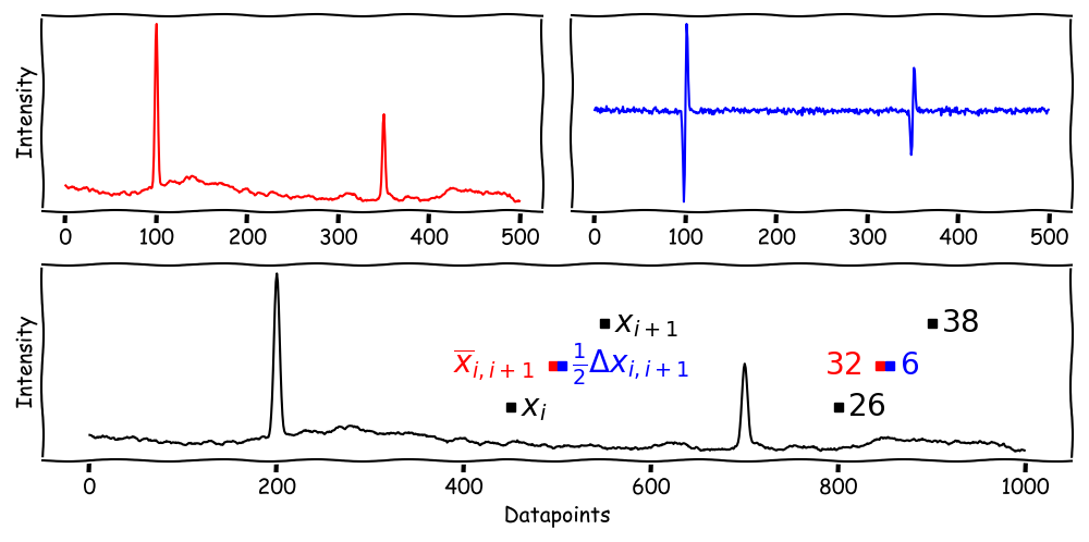
Savitzky-Golay: 1st Derivative
The 1st derivative provides both smoothing and baseline correction by highlighting changes in the signal while reducing noise.
How it works: Savitzky-Golay computes derivatives directly from a polynomial fit within a moving window.
Applications:
Removing baseline drifts by zeroing the derivative of constant or linear trends.
Smoothing noisy data while retaining peak features and enhancing changes.
Example Polynomial Fit: \[ y'(t) = \frac{d}{dt} \sum_{i=-n}^{n} c_i \cdot f(t + i) \]
Figure: solid blue line is the original signal, solid black line is the smoothed signal, and dashed black line is the 1st derivative. The red dashed line shows the conventional derivative without smoothing.
Savitzky-Golay: Generating Coefficients
How are Savitzky-Golay Coefficients generated?
The coefficients are derived by fitting a polynomial over a moving window using a Vandermonde matrix and its pseudo-inverse.
Vandermonde Matrix:
(e.g., for 5 points & 2 orders)
\[
\mathbf{V} =
\begin{bmatrix}
1 & t_{-2} & t_{-2}^2 \\
1 & t_{-1} & t_{-1}^2 \\
1 & t_{0} & t_{0}^2 \\
1 & t_{1} & t_{1}^2 \\
1 & t_{2} & t_{2}^2
\end{bmatrix}
=
\begin{bmatrix}
1 & -2 & 4 \\
1 & -1 & 1 \\
1 & 0 & 0 \\
1 & 1 & 1 \\
1 & 2 & 4
\end{bmatrix}
\]
where \( t_i \in \{-2, -1, 0, 1, 2\} \) for a window of 5 points.
Pseudo-Inverse: \[ \mathbf{V}^+ = (\mathbf{V}^T \mathbf{V})^{-1} \mathbf{V}^T \] The rows of \( \mathbf{V}^+ \) are the coefficients for smoothing and derivatives.
Extract Coefficients:
\[
\mathbf{V}^+ =
\begin{bmatrix}
-3 & 12 & 17 & 12 & -3 \\
-2 & -1 & 0 & 1 & 2 \\
1 & -2 & 0 & 2 & -1
\end{bmatrix}
\]
# 1st Row (Normalized): For smoothing.
# 2nd Row: For the 1st derivative.
# 3rd Row: For the 2nd derivative.
Normalization: The 1st row (for smoothing) must be normalized: \[ c_i^{\text{norm}} = \frac{c_i}{\sum_j c_j} \] Resulting in: \[ c^{\text{norm}} = \left[ -0.086, 0.343, 0.486, 0.343, -0.086 \right] \]
Relevance of Other Rows:
1st Row: Weighted mean for smoothing.
2nd Row: Approximates the 1st derivative (scaled by \( 1/\Delta t \)).
3rd Row: Approximates the 2nd derivative (scaled by \( 1/\Delta t^2 \)).
Denoising using Fourier Transformation
What is Fourier Transformation and how does it work?
Fourier Transformation transfers axial frequencies to radial frequencies and analyzes interferences.
Axial Frequency:
Periodic signal along an axis.
\[
\cos(x \cdot f)
\]
Frequency:
10
Interference:
Multiple frequencies can be combined to create interferences.
\[
\cos(x \cdot f_1) + \cos(x \cdot f_2)
\]
Frequency 1:
10
Frequency 2:
20
Denoising using Fourier Transformation
Radial:
Number of loops around a circle.
\[
\exp(i \cdot x \cdot f)
\]
The radial frequency is the number of loops around the circle per unit of time.
Interference:
Combining axial and radial frequencies.
\[
\exp(i \cdot x \cdot f) \cdot \cos(x \cdot f)
\]
Denoising using Fourier Transformation
Fourier Transformation combines axial and radial frequencies to identify patterns: \[ \hat{y}_k = \sum_{j=0}^{N-1} \left(e^{-2\pi i \cdot \frac{jk}{N}} \cdot y_j\right) \] Where \( y \) is the dataset with \( N \) points.
When frequencies differ, the integral approaches zero. For matching frequencies, the sum increases.
Circle Frequency: 1
The integral can be interpreted as the distance between geometric mean of the dataset to the origin of the cooordinate system, which is shown in blue.
The dinstance maximizes when the frequencies match.
Systematic Frequency Analysis
Fourier Transformation systematically varies radial frequencies to identify all frequencies in the dataset.
This process works in both directions and is reversible:
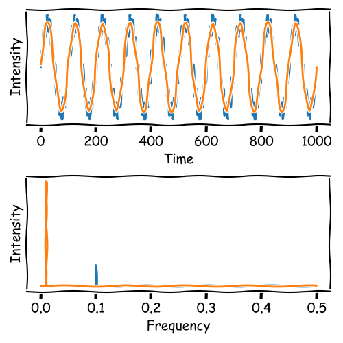
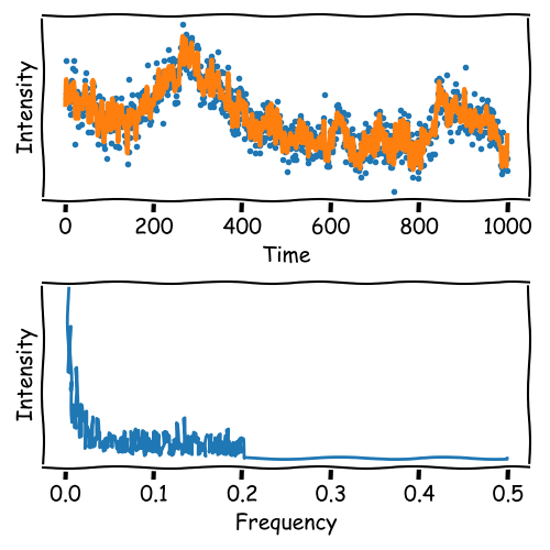
Frequency Filtering
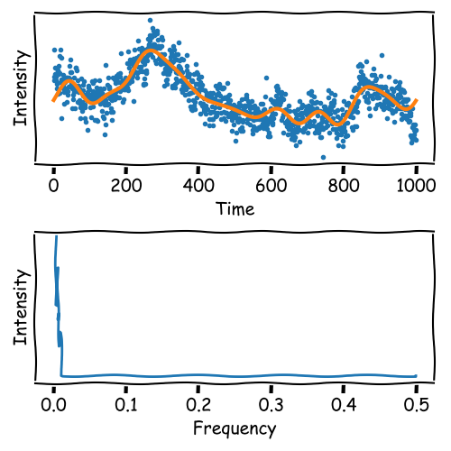
High-frequency noise can be filtered by removing frequencies above a threshold:
\[ I(f) = \begin{cases} I(f), & \text{if } f < \text{threshold} \\ 0, & \text{otherwise.} \end{cases} \]
The result is a denoised dataset.
Frequency Filtering
Frequency Filtering
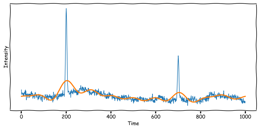
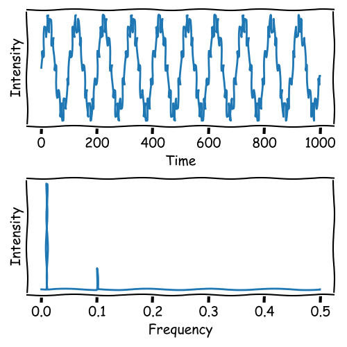
When the signal contains sharp peaks, the Fourier Transformation may not be suitable for denoising.
Sharp peaks contain high-frequency components that are essential for the signal.
Frequency Filtering
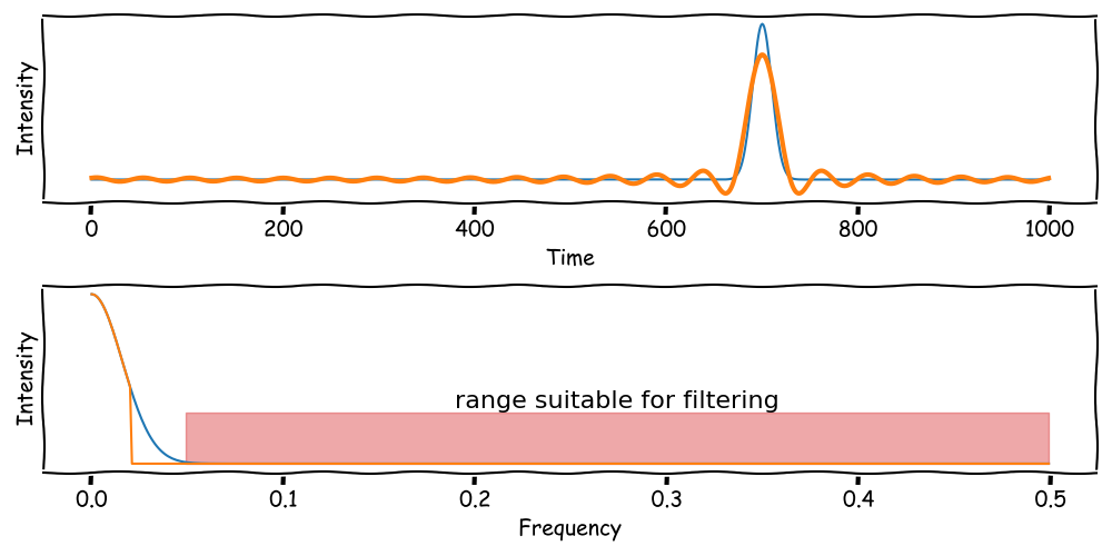
Peaks contain not a single frequency but a range of frequencies.
The sharper the peak, the broader the frequency range.
This band from the peak limits the effectiveness of frequency filtering.
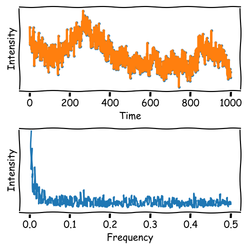
Frequency Filtering
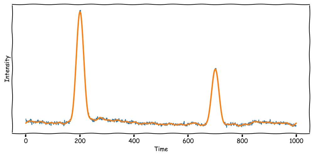
When the signal contains broad peaks, the Fourier Transformation may be suitable for denoising.
Broad peaks contain leave more room for frequency filtering.
Fourier Transformation Summary
Fourier Transformation extracts frequencies from a signal: \[ \hat{y}_k = \sum_{j=0}^{N-1} \left(e^{-2\pi i \cdot \frac{jk}{N}} \cdot y_j\right) \] Output: Frequency spectrum showing which frequencies are present in the signal.
Frequencies can be filtered (e.g., high-frequency noise removal).
The signal can be transformed back to the time domain after filtering.
Key Limitation:
Fourier Transformation does not provide information about where a frequency occurs in the dataset.
Advantage:
Fourier Transformation uses that noise is often high-frequency and can be filtered out.
Alternative:
Discrete Wavelet Transformation provides information about the location of frequencies.
Discrete Wavelet Transformation Introduction
Discrete Wavelet Transformation (DWT):
A method that decomposes a signal into components using wavelets.
Unlike FFT, DWT provides both frequency and location information of the signal's features.
\[ DWT(x) = \sum_{j,k} x(t) \cdot \psi_{j,k}(t) \] Where \(\psi_{j,k}(t)\) are scaled and shifted versions of a mother wavelet.
Wavelets are localized in both time and frequency.
Comparison:
- FFT: Great for extracting global frequencies, but no location info.
- DWT: Ideal for detecting transient features and changes over time.
What is a Wavelet?
A wavelet is a kernel function with a specific shape and properties, e.g., sum of all values is zero.
Wavelets are used to analyze signals at different scales, i.e. resolutions.
The most simple wavelet is the Haar wavelet.
\[
\psi(t) = \begin{cases} 1, & 0 \leq t < 0.5 \\ -1, & 0.5 \leq t < 1 \end{cases}
\]
The Haar Wavelet
In DWT, we use two functions to analyze signals.
The Haar wavelet operates on two functions:
1. Scaling Function (\(\phi(t)\)):
Used to calculate averages (low-frequency components).
\[
\phi(t) = \begin{cases} 1, & 0 \leq t < 1 \\ 0, & \text{otherwise.} \end{cases}
\]
2. Wavelet Function (\(\psi(t)\)):
Used to calculate differences (high-frequency components).
\[
\psi(t) = \begin{cases} 1, & 0 \leq t < 0.5 \\ -1, & 0.5 \leq t < 1 \\ 0, & \text{otherwise.} \end{cases}
\]
These functions decompose a signal into approximations and details.
Haar Wavelet Examples on Different Scales:
Haar Wavelet Transformation Step-by-Step
The Haar Wavelet Transformation processes data by:
1. Splitting the data \( y \) into vertical packages: (e.g., scale of 4) \[ y = \begin{bmatrix} y_1 \\ y_2 \\ y_3 \\ y_4 \\ \vdots \\ y_n \end{bmatrix} \rightarrow P = \begin{bmatrix} y_1 & y_{5} & y_{9} \\ y_2 & y_{6} & y_{10} \\ y_3 & y_{7} & y_{11} \\ y_4 & y_{8} & y_{12} \end{bmatrix} \]
2. Applying the Scaling Function: \[ \phi = \frac{1}{4} \begin{bmatrix} 1 & 1 & 1 & 1 \end{bmatrix} \] Averages: \[ A = \phi \cdot P \]
3. Applying the Wavelet Function: \[ \psi = \frac{1}{4} \begin{bmatrix} 1 & 1 & -1 & -1 \end{bmatrix} \] Differences: \[ D = \psi \cdot P \]
4. Recursive Process: with a constant scale of 2, the process is repeated until the desired
P -> A1 & D1
      ↳ A2 & D2
         ↳ A3 & D3
            ↳ A4 & D4
Example of DWT
The DWT decomposes a signal into approximations and details.
Approximations represent the signal's low-frequency components (father wavelet).
Details represent the signal's high-frequency components (mother wavelet).
DWT and the Multi Resolution Analysis
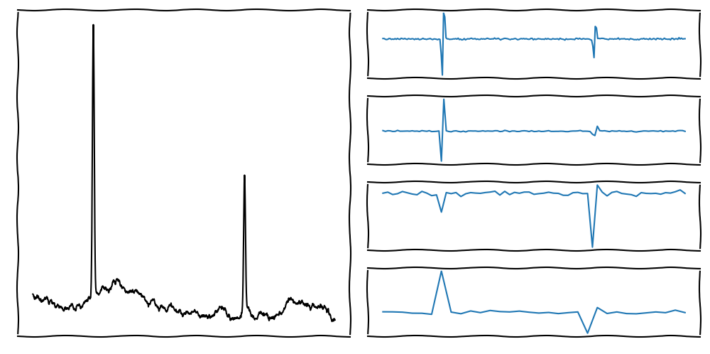
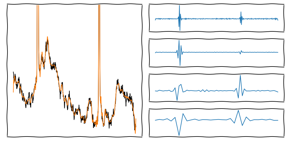
On the left side, we see the original signal.
On the right side, we see the Details of multiple scales (steps)
The indivudal Details describe the signal's frequencies at different scales (high scale = low frequency).
DWT and the Multi Resolution Analysis
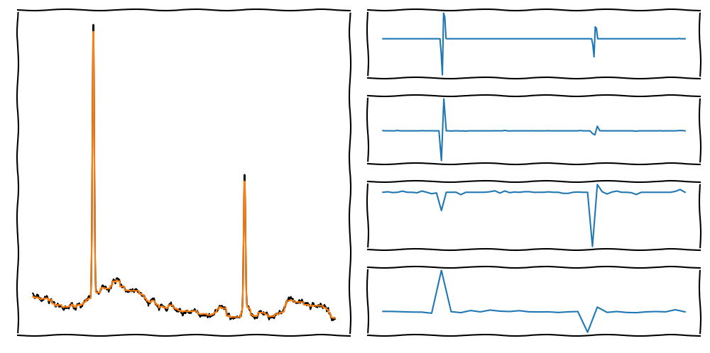
On the left side, we see the original and reconstructed signal.
To denoise, we use filters on the different scales (Details).
The reconstructed signal is the sum of the approximations and the filtered details.
DWT and the Multi Resolution Analysis
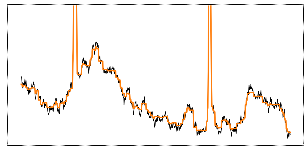
Depending on the Wavelet, the signal may look step-like (e.g., Haar Wavelet).
To improve the reconstruction, we can use different Wavelets.
DWT and the Multi Resolution Analysis
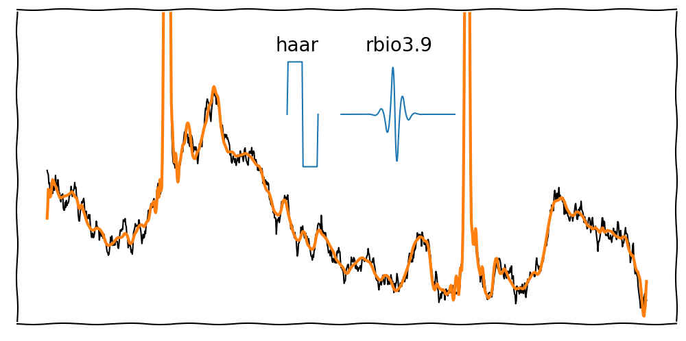
Depending on the Wavelet, the signal may look step-like (e.g., Haar Wavelet).
There are many Wavelets available, e.g., rbio3.9 or db4. Each Wavelet has different strengths and weaknesses.
DWT and the Multi Resolution Analysis
On the left side, we see the original and reconstructed signal.
To denoise, we use filters on the different scales (Details).
The reconstructed signal is the sum of the approximations and the filtered details.
Discrete Wavelet Transformation Summary
The Discrete Wavelet Transformation (DWT) provides a way to analyze signals in both:
Frequency domain (like FFT).
Time domain (unlike FFT).
By using Wavelets:
Approximations: Low-frequency components for trends (smooth signal).
Details: High-frequency components for transient features (sharp changes).
Advantages of DWT:
Detects location of features in the signal.
Supports multi-resolution analysis (analyzing signals at different scales).
Key Applications:
- Noise reduction (denoising).
- Image compression (e.g., JPEG 2000).
- Transient detection (e.g., ECG or fault detection).