Chemometrics & Statistics
08. Data Modeling 3Machine Learning
Initial Thoughts on Machine Learning
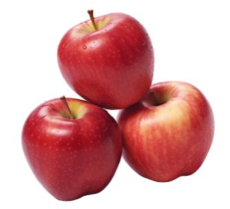
What is shown in the image?
Describe how you draw your conclusion.
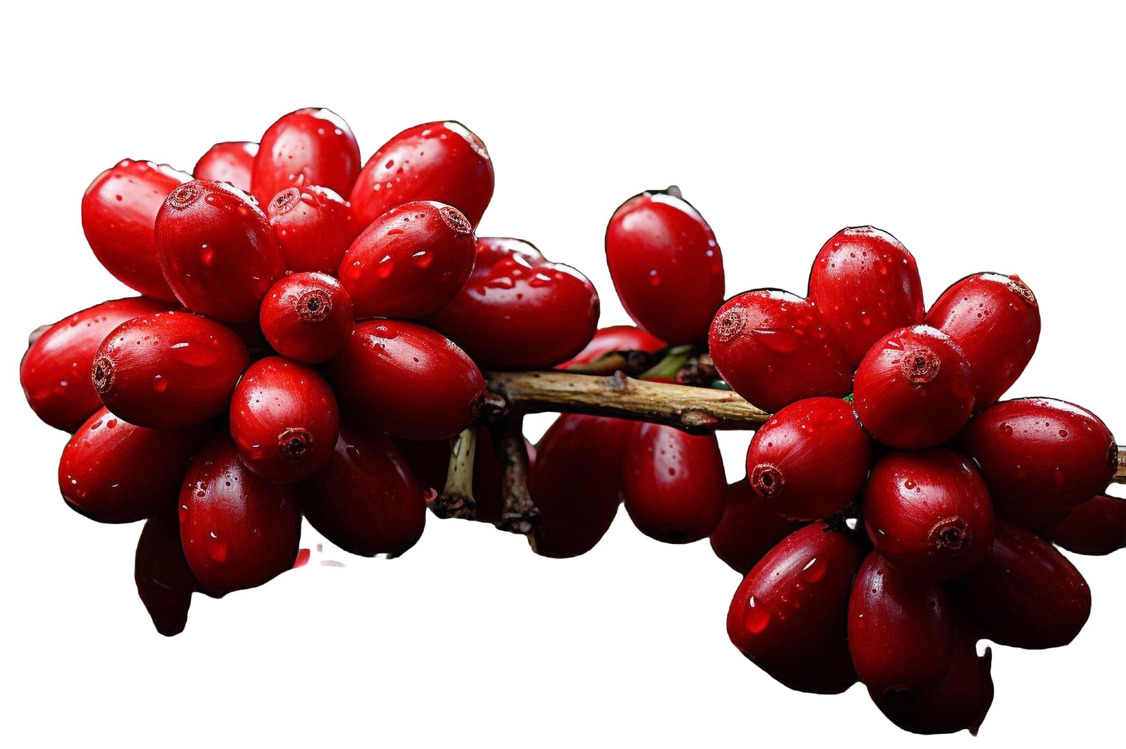
Initial Thoughts on Machine Learning

What is shown in the image?
Describe how you draw your conclusion.
Initial Thoughts on Machine Learning
What is shown in the image?
Describe how you draw your conclusion.
Initial Thoughts on Machine Learning
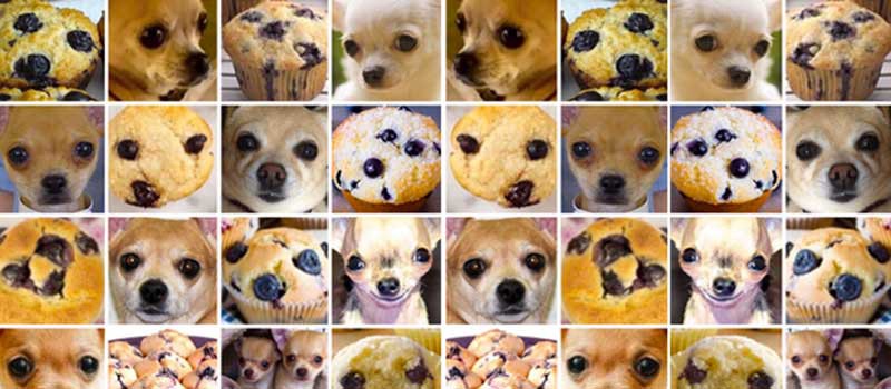
Can we classify the images as dogs or muffins?
Describe how you draw your conclusion.
Insights from Initial Thoughts
Humans recognize patterns instinctively:
We rely on prior knowledge (e.g., apples, dragon fruit).
Familiar features like color, texture, and shape help us make decisions.
Some classifications are straightforward:
Distinctive features make certain objects easy to identify.
Some classifications are challenging:
We do not have prior knowledge (e.g., coffee beans).
Ambiguity is a challenge:
Overlap in features (e.g., dogs vs. muffins) creates confusion.
Machine Learning's key questions:
How can algorithms recognize patterns like humans? characteristic features
How can ambiguity and errors be reduced? high quality data
What is Machine Learning?
Definition:
Machine Learning is a subset of Artificial Intelligence (AI) that enables systems to learn and improve
from data without explicit programming.
Objectives of ML:
Classification
Predicting discrete categories, e.g., identifying spam emails, or classifying water quality.
Regression
Predicting continuous values, e.g., forecasting house prices, or estimating chemical concentrations.
Types of ML:
Supervised Learning
Learning from labeled data, e.g., classifying images as "cat" or "dog" or predicting blood glucose
levels. Reference data
Unsupervised Learning
Finding hidden patterns in unlabeled data, e.g., customer segmentation or anomaly detection. No reference data
Reinforcement Learning
Learning by interacting with an environment, e.g., training robots or game-playing AI. Feedback from environment
Important Terms in ML
Features:
Input variables that describe the data, e.g., temperature, pH, turbidity in water quality analysis.
Labels:
Output variables that define the target, e.g., "potable" or "non-potable" in water quality classification.
Training Data:
Dataset used to train the model, consisting of features and labels.
Model:
Algorithm that learns patterns from training data to make predictions.
Testing Data:
Dataset used to evaluate the model's performance on unseen data.
Metrics:
Measures used to assess model performance, e.g., accuracy.
Complexity, Generalization, and Over- & Underfitting
Underfitting: Model is too simple, fails to capture patterns (high bias).
Overfitting: Model is too complex, captures noise instead of patterns (high variance).
Generalization: Balance between bias and variance, enabling good performance on unseen data.
.png)
.png)
.png)
Balancing Model Complexity: A trade-off between underfitting and overfitting.
The principle of Logistic Regression
What is Logistic Regression?
A statistical method used to predict the probability of a binary outcome (e.g., yes/no, 0/1).
How does it work?
Maps input variables to probabilities using the sigmoid function:
P = 1 / (1 + exp(-z)) , where z is a linear combination of inputs.
Applications, Pros, and Cons of Logistic Regression
Applications:
Environmental Toxicology:
a) Predicting acute toxicity levels in water samples based on chemical concentrations.
Water Quality Monitoring:
a) Classifying water samples as "potable" or "non-potable" based on parameters like turbidity,
conductivity, and bacterial count.
b) Identifying pollution sources by classifying samples into "industrial" vs. "agricultural"
contamination.
Pros:
Simple and interpretable, works well for linearly separable data.
Cons:
Limited to binary outcomes, struggles with non-linear relationships and outliers.
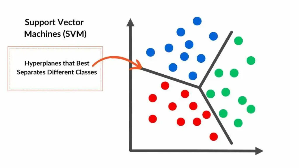
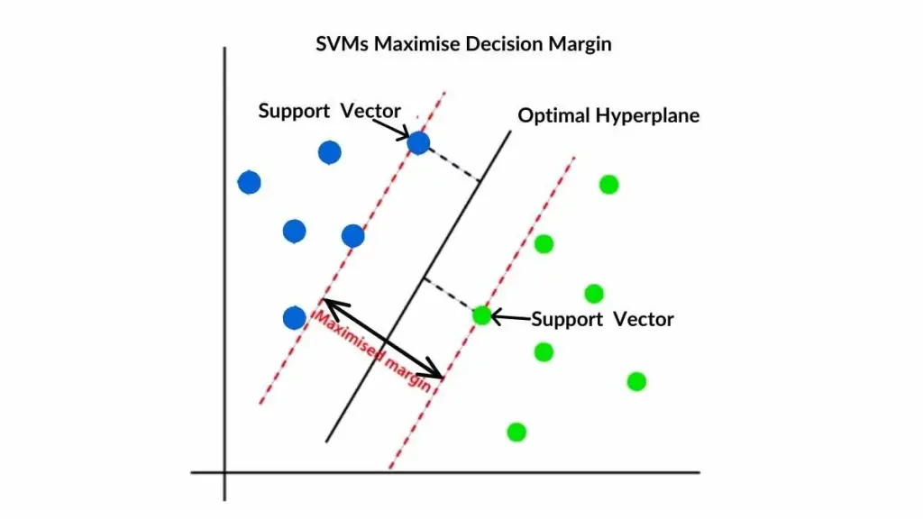
The principle of Support Vector Machines
What is a Support Vector Machine?
A supervised machine learning algorithm used for classification and regression tasks.
How does it work?
SVMs find the hyperplane that best separates data points into different classes, maximizing the margin between the closest points (support vectors) of each class.
https://spotintelligence.com/2024/05/06/support-vector-machines-svm/
Applications, Pros, and Cons of Support Vector Machines
Applications:
Environmental Toxicology:
a) Classifying pollutants in water samples based on chemical fingerprints.
Water Quality Monitoring:
a) Detecting harmful algae blooms by analyzing spectral data.
b) Identifying contamination sources using multi-parameter datasets.
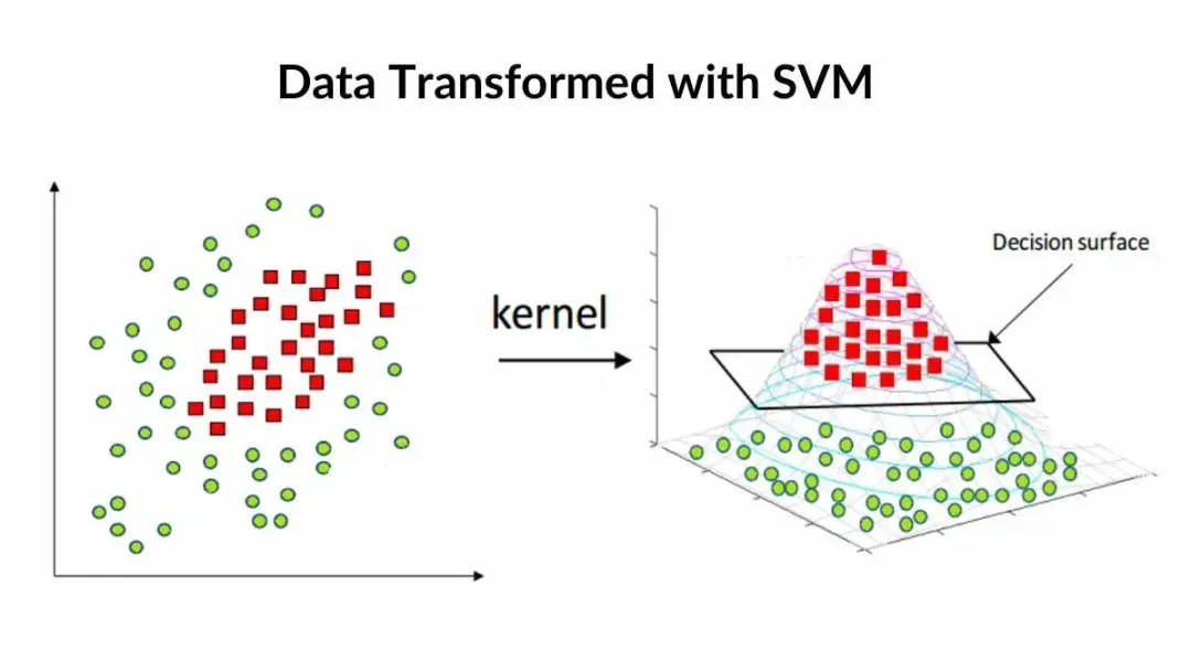
Pros:
Effective for high-dimensional spaces, works well with non-linear data using kernel trick.
https://spotintelligence.com/2024/05/06/support-vector-machines-svm/
Cons:
Computationally expensive for large datasets, sensitive to choice of kernel and hyperparameters.
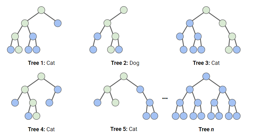
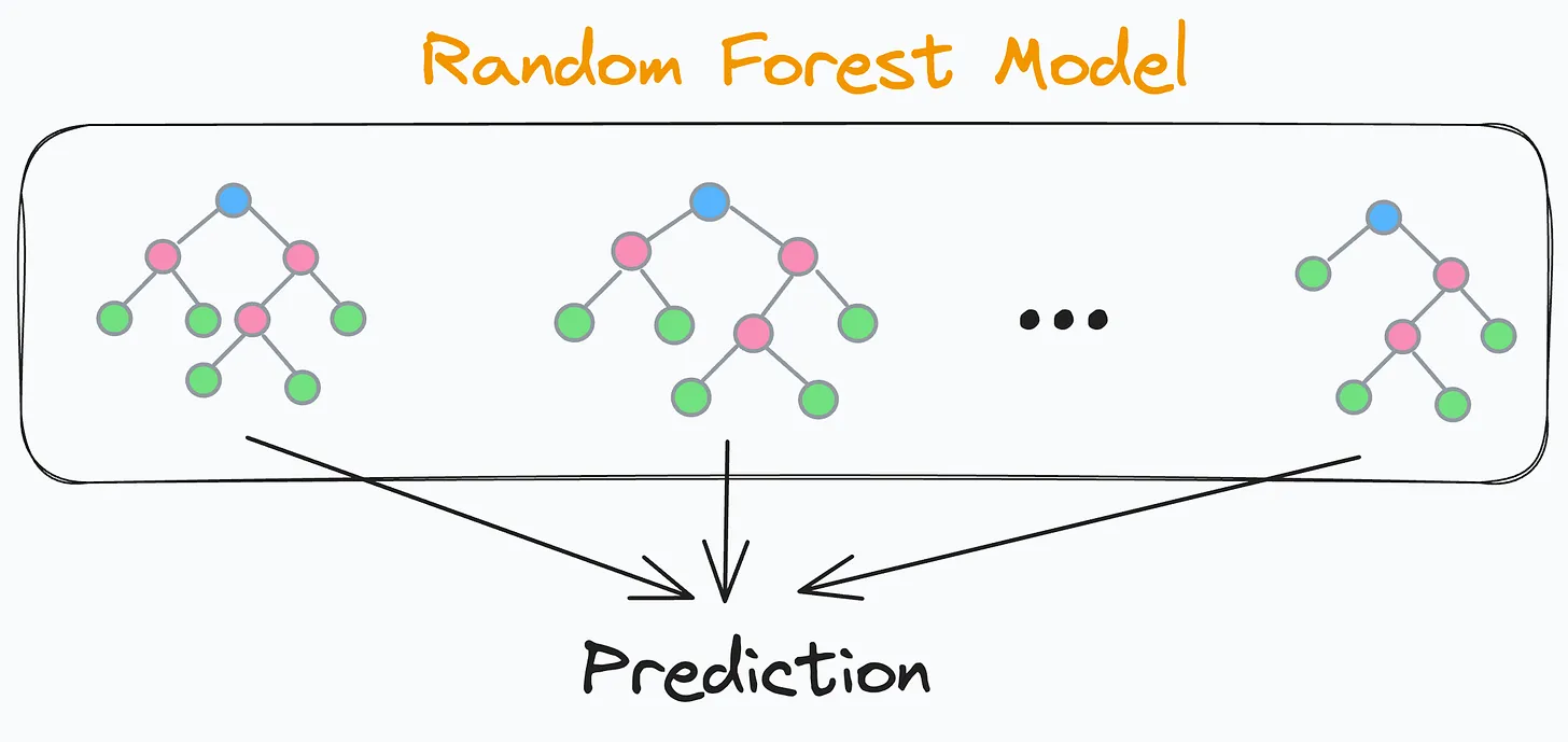
The principle of Random Forest
What is Random Forest?
An ensemble learning method that combines multiple decision trees to improve accuracy and reduce overfitting.
Key Features:
Uses bootstrapping and random feature selection.
Aggregates outputs (majority vote for classification, average for regression).
Random Forest Scheme (https://www.datacamp.com/de/tutorial/random-forests-classifier-python)
What is a Decision Tree?
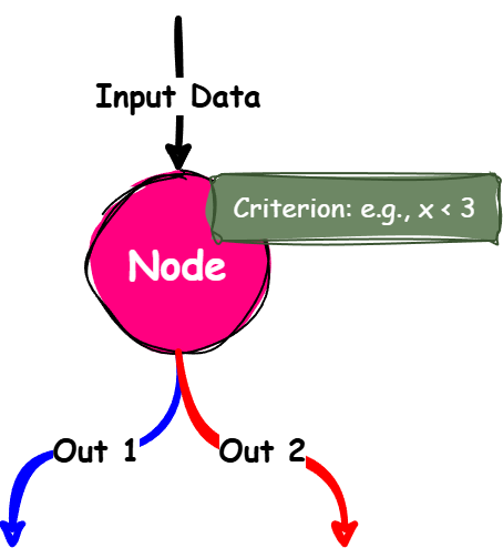
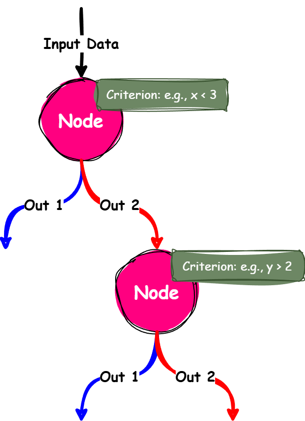
What is a Decision Tree?
A tree-like model for making decisions based on splitting data by specific criteria.
How it works:
a) Splits data based on a feature and threshold to maximize separation.
b) Grows branches until a stopping criterion is met (e.g., min samples or max depth).
Components of a Decision Tree:
Root Node: Represents the entire dataset and the first split.
Decision Nodes: Points where the data is split further.
Leaf Nodes: Terminal nodes showing the final result.
Branches: Connect nodes and represent the outcome of a decision.
What is an Ensemble Approach?
Definition:
Combining predictions from multiple decision trees to improve overall model performance.
How it works:
Builds multiple decision trees from different subsets of data.
Each tree contributes a vote (classification) or prediction (regression).
The final output is based on majority vote (classification) or average (regression).
Example in RF:
                  Tree 1: Class A
                  Tree 2: Class B
                  Tree 3: Class A
                  Final Prediction: Majority vote = Class A

                  Regression:
                  Tree 1: 5.2
                  Tree 2: 5.5
                  Tree 3: 5.1
                  Final Prediction: Average = 5.27
Why use an ensemble?
Reduces overfitting by averaging predictions.
Improves robustness and accuracy.
Handles noisy data better than a single tree.
What is Boot Strap Sampling in RF?
Definition:
Resampling technique used to create subsets of data for training individual decision trees.
Idea behind Bootstrapping:
From a dataset of size N, create multiple subsets of size N by randomly sampling with replacement.
Why it matters:
a) Ensures diversity in decision trees.
b) Provides built-in validation using out-of-bag samples.
In Practice:
          original_dataset = [1, 2, 3, 4, 5]
          bootstrapped_tree1 = [2, 4, 5, 1, 2]
          bootstrapped_tree2 = [3, 5, 1, 3, 3]
          oob_sample_tree1 = [3]
          oob_sample_tree2 = [2, 4]
How many trees are built?
Typically, hundreds to thousands of trees are trained in a Random Forest.
It is a hyperparameter that can be optimized.
Example:
x = [1, 2, 3, 4, 5, 6, 7, 8, 9, 10]
How to set up an RF?
Structure of a Random Forest:
Composed of multiple decision trees.
Each tree is trained on a unique bootstrapped dataset.
Not only the data but also the features are randomly sampled for each node in each tree.
Feature that provides the best split of the data is selected.
Trees grow independently until a stopping condition (e.g., max depth, min samples per leaf).
Random Forest Scheme (https://blog.dailydoseofds.com/p/your-random-forest-is-underperforming)
Key Features:
Combines outputs of trees using majority vote (classification) or averaging (regression).
Randomness ensures diversity in trees, reducing overfitting.
Out-of-bag (OOB) samples can validate model performance.
Find the best Criterion for a Knot
Choosing the Best Feature:
At each node, a random subset of features is selected from the total features.
Each feature in the subset is evaluated to determine the best split for the data.
Criterion for Splitting:
Common criteria evaluate purity of the resulting child nodes after a split.
For classification:
Gini Index: Measures impurity. Lower values are better.
\[ Gini = 1 - \sum_{i=1}^{n} p_i^2 \]
where p is the proportion of samples in class i.
For regression:
Mean Squared Error (MSE): Evaluates the reduction in variance after a split.
How the Best Criterion is Determined:
For each feature and potential split point, calculate the criterion value.
Choose the split point that maximizes the improvement in purity or minimizes the error.)
Example:
Feature Subset: [Turbidity, Conductivity, pH]
Turbidity (GI) | Conductivity (GI) | pH (GI)
  < 5.0: 0.2   |  < 100: 0.1       |  < 7.0: 0.3
  < 5.2: 0.3   |  < 150: 0.2       |  < 7.2: 0.2
  < 5.5: 0.4   |  < 200: 0.3       |  < 7.5: 0.4
  < 6.0: 0.8   |  < 250: 0.4       |  < 8.0: 0.2

Best Split: Conductivity < 100 (Gini Index = 0.1)
Why it Matters:
Ensures the tree makes the most informative splits, leading to accurate predictions.
Balances complexity and data splitting quality.
Example for Gini Index
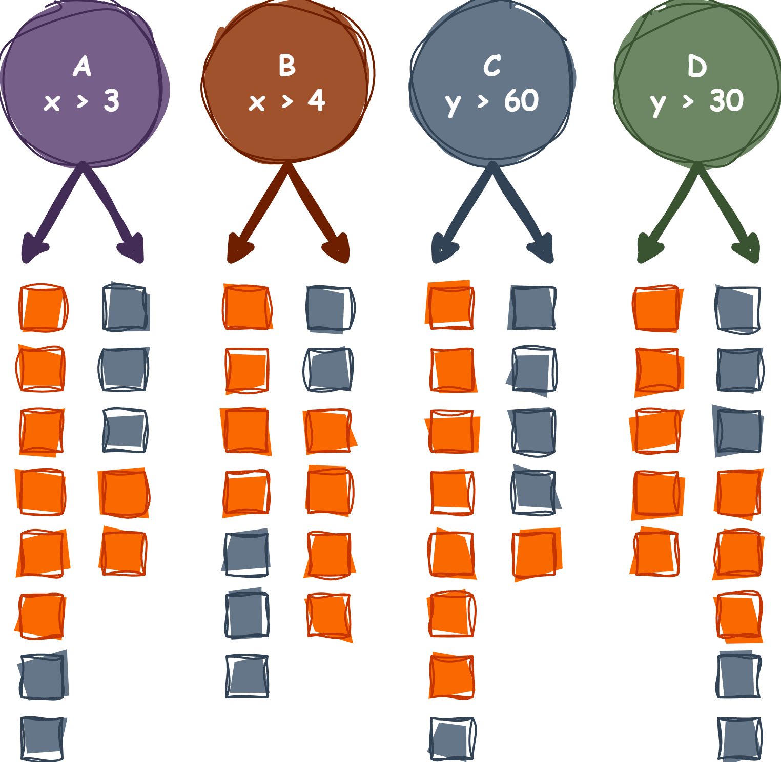
Possible splits for a decision tree node.
A: out1 (5, 2); out2 (2, 3) \[ Gini_1 = 1 - \left( \left( \frac{6}{7} \right)^2 + \left( \frac{2}{7} \right)^2 \right) \approx 0.375 \] \[ Gini_2 = 1 - \left( \left( \frac{2}{5} \right)^2 + \left( \frac{3}{5} \right)^2 \right) = 0.48 \] \[ Gini_{\text{split}} = \frac{n_1}{n} \times Gini_1 + \frac{n_2}{n} \times Gini_2 \] \[ Gini_{\text{split}} = \frac{8}{13} \times 0.375 + \frac{5}{13} \times 0.48 \approx 0.42 \]
Other Splits:
B) Gini Index: 0.47
C) Gini Index: 0.26
D) Gini Index: 0.29
What if I have Multiple classes?
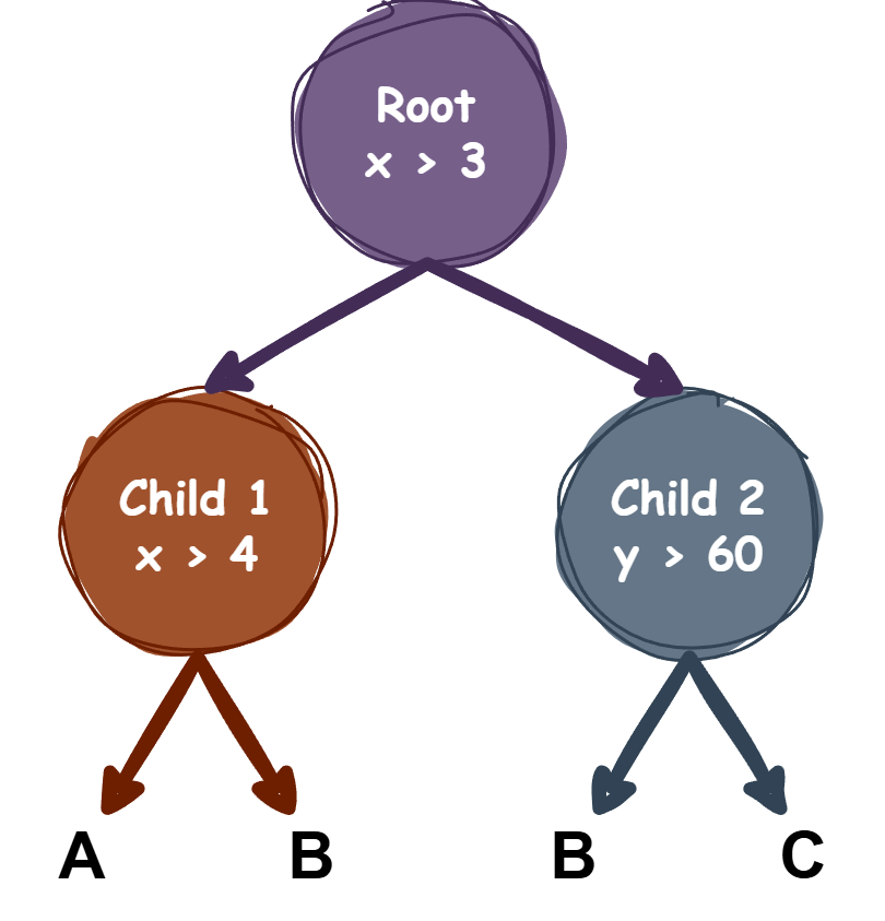
Handling Multiple Classes:
A Decision Tree can handle multiple classes as the Gini Index can be extended to multi-class problems.
This will lead to a cascade of binary splits to separate the classes.
Example:
Classes: A, B, C
Root node: mainly separated into A and not A.
Child node 1: further clean A into A and B.
Child node 2: further clean not A into B and C.
Understanding Feature Importance in RF
What is Feature Importance?
A measure of how valuable each feature is for improving the model's performance.
How is it calculated?
Impurity-Based Importance: Sum of impurity reduction (e.g., Gini Index or MSE) for splits using the feature. \[ \text{Importance of feat.} = \sum_{\text{all trees}} \sum_{\text{all nodes}} \text{Impurity Reduction} \div \text{Total Impurity Reduction} \]
Permutation Importance: Decrease in model performance when feature values are shuffled.
Why is it important?
Identifies which features contribute most to predictions, aiding interpretability and model refinement.
Example:
Feature Importance:
Turbidity: 0.7
pH: 0.2
Conductivity: 0.1
Random Forest Example: Classification
Problem:
Classify water samples as "Potable" or "Non-Potable" based on turbidity, conductivity, and pH.
Turbidity | Conductivity | pH | Class
-------------------------------------
  5.0    |  100        |  7.0 | Potable
  5.2    |  150        |  7.2 | Non-Potable
  5.5    |  200        |  7.5 | Potable
  6.0    |  250        |  8.0 | Non-Potable
-------------------------------------
unknown samples:
  5.2    |  160        |  7.1 | ?
  6.5    |  300        |  8.5 | ?
Step 1: Set Up Decision Trees
Let's build 5 decision trees using bootstrapped samples and random feature selection.
bootstrap_sample1 =
  [5.0, 100, 7.0, Potable]
  [5.0, 100, 7.0, Potable]
  [6.0, 250, 8.0, Non-Potable]
  [6.0, 250, 8.0, Non-Potable]

bootstrap_sample2 = ...
Step 2: Train Trees
Train each tree on a bootstrapped sample.
Tree 1:
Root Node: Conductivity < 250 (Gini = 0.0)
No further splits needed (Purity = 100%)
OOB Samples for validation:
[5.2, 150, 7.2, Non-Potable] -> Predicted: Potable
[5.5, 200, 7.5, Potable] -> Predicted: Potable

Tree 2: ...
Validation and Feature Importance
Validate model performance by using out-of-bag samples.
Out-of-Bag Samples:
T1: [5.2, 150, 7.2, Non-Potable] -> Potable
T1: [5.5, 200, 7.5, Potable] -> Potable
T2: [5.0, 100, 7.0, Potable] -> Potable
T3: [6.0, 250, 8.0, Non-Potable] -> Non-Potable
Error Rate: 25%
Feature Importance:
  Conductivity = 0.3
  Turbidity = 0.6
  pH = 0.1
Final Prediction
Combine tree predictions using majority vote.
Unkown Sample 1: [5.2, 160, 7.1]
  Votes: Potable, Potable, Non-Potable
  = Potable
Unkown Sample 2: [6.5, 300, 8.5]
  Votes: Non-Potable, Non-Potable, Non-Potable
  = Non-Potable