Chemometrics & Statistics
07. Data Modeling 2Non-Linear Regression
What is the Leverage Effect in Regression?
Introduction:
The leverage effect measures how far an observation's predictor values are from the mean of all predictor values.
Observations with high leverage have the potential to exert significant influence on the estimated regression coefficients.
Understanding leverage is crucial for identifying influential data points and ensuring the robustness of your regression model.
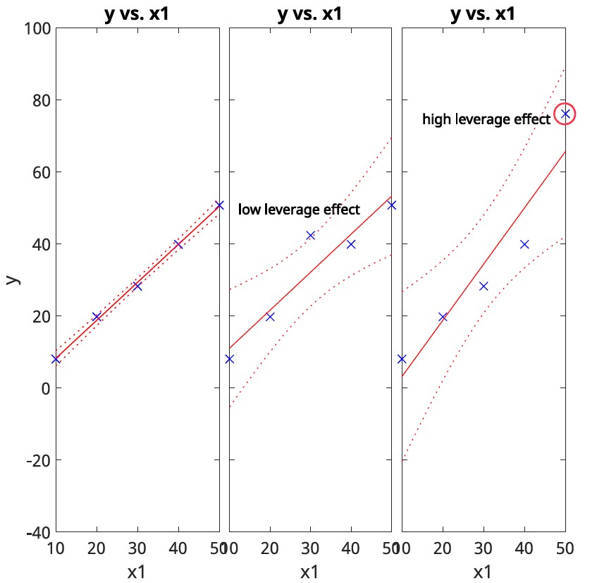
High leverage points significantly influence the regression model, i.e., regression coefficients.
Mathematical Foundations of the Leverage Effect
The Hat Matrix (\(\mathbf{H}\)):
The leverage of each observation is given by the diagonal elements \(h_{ii}\) of the Hat Matrix: \[ \mathbf{H} = \mathbf{X} (\mathbf{X}^\top \mathbf{X})^{-1} \mathbf{X}^\top \]
Properties of \(h_{ii}\):
\(0 \leq h_{ii} \leq 1\)
\(\sum_{i=1}^{n} h_{ii} = p\) (number of parameters)
Interpretation:
A high leverage value \(h_{ii}\) indicates that observation \(i\) is far from the mean of the predictor variables.
Such observations can significantly influence the estimated regression coefficients.
Example:
\[ \mathbf{X} = \begin{pmatrix} 1 & 1 & 1 \\ 1 & 2 & 4 \\ 1 & 3 & 9 \\ 1 & 4 & 16 \\ 1 & 5 & 25 \\ \end{pmatrix} \quad \mathbf{H} = \begin{pmatrix} .9 & . & . & . & . \\ . & .4 & . & . & . \\ . & . & .5 & . & . \\ . & . & . & .4 & . \\ . & . & . & . & .9 \\ \end{pmatrix} \] The diagonal elements of \(\mathbf{H}\) are the leverage values.
Interpretation of Leverage Values \(h_{ii}\)
High Leverage Indicates:
An observation with a high leverage value \(h_{ii}\) is far from the mean of the predictor variables.
Identifying High Leverage Points:
A commonly used threshold: \[ h_{ii} > \frac{2p}{n} \]
where \(p\) is the number of parameters and \(n\) is the number of observations.
Observations beyond the threshold are considered high-leverage points.
Example:
a) Equidistant predictor values: \[ thr = .8 \quad \mathbf{X} = \begin{pmatrix} 1 & 10 \\ 1 & 20 \\ 1 & 30 \\ 1 & 40 \\ 1 & 50 \\ \end{pmatrix} \quad \text{diag}\left(\mathbf{H}\right) = \begin{pmatrix} .6 \\ .3 \\ .2 \\ .3 \\ .6 \\ \end{pmatrix} \quad \checkmark \] b) Non-equidistant predictor values: \[ \mathbf{X} = \begin{pmatrix} 1 & 1 \\ 1 & 2 \\ 1 & 5 \\ 1 & 10 \\ 1 & 50 \\ \end{pmatrix} \quad \text{diag}\left(\mathbf{H}\right) = \begin{pmatrix} .3 \\ .3 \\ .2 \\ .2 \\ 1. \\ \end{pmatrix} \quad \text{⚠︎} \]
Practical Implications:
High-leverage points may not necessarily be outliers in the response variable but can disproportionately affect the regression model.
Relationship between Leverage and Influence
Influence of an Observation:
depends on both its leverage and its residual.
an observation with high leverage and a large residual can have a significant impact on the regression model.
Cook's Distance (\(D_i\)):
measures the influence of an observation: \[ D_i = \frac{(e_i)^2}{p \cdot \hat{\sigma}^2} \frac{h_{ii}}{(1 - h_{ii})^2} \]
where \(e_i\) is the residual of observation \(i\), \(p\) is the number of parameters, and \(\hat{\sigma}^2\) is the estimated variance.
Interpretation of Cook's Distance:
A larger \(D_i\) indicates a more influential observation.
Common threshold: \[ D_i > \frac{4}{n} \] where \(n\) is the number of observations.
Calculation Example: Cook's Distance
Case 1: Low Leverage Outlier
Dataset:
\[ \begin{array}{c|ccccc} x_i & 1 & 2 & 5 & 10 & 50 \\ y_i & 1.6 & 2.0 & 5.4 & 4.3 & 15.6 \\ \end{array} \]
Steps:
Fit the regression model \(y = \beta_0 + \beta_1 x\)
Compute residuals \(e_i\) and leverage values \(h_{ii}\)
Calculate Cook's Distance \(D_i\) for each observation
Cook's Distance \(D_i\):
\[ \begin{array}{c|ccccc} \text{Observation} & 1 & 2 & 3 & 4 & 5 \\ \hline D_i & 0.10 & 0.06 & 0.48 & 0.03 & 1.37 \\ \end{array} \]
Case 2: High Leverage Outlier
Dataset:
\[ \begin{array}{c|ccccc} x_i & 1 & 2 & 5 & 10 & 50 \\ y_i & 1.6 & 2.0 & 2.7 & 4.3 & 22.1 \\ \end{array} \]
Steps:
Fit the regression model \(y = \beta_0 + \beta_1 x\)
Compute residuals \(e_i\) and leverage values \(h_{ii}\)
Calculate Cook's Distance \(D_i\) for each observation
Cook's Distance \(D_i\):
\[ \begin{array}{c|ccccc} \text{Observation} & 1 & 2 & 3 & 4 & 5 \\ \hline D_i & 0.17 & 0.12 & 0.03 & 0.29 & 62.50 \\ \end{array} \]
Conclusions: The Leverage Effect in Regression
Key Takeaways:
The leverage effect measures how far an observation's predictors are from the mean.
High-leverage points can significantly influence regression coefficients.
Cook's Distance measures observation influence using leverage and residuals.
Practical Implications:
Identifying influential points ensures robust regression analysis.
Such points may indicate errors, outliers, or important data variations.
Conclusions for Experimental Design:
Data Quality: Check for errors or anomalies causing high leverage.
Balanced Design: Plan experiments to minimize unintended high leverage.
Robustness Checks: Use diagnostics (e.g., Cook's Distance) to assess influence.
Decision Making: Consider context when deciding on influential points.
Mitigating the Leverage Effect with Weighted Regression
Weighted Regression with Cook's Distance
Assign weights inversely related to Cook's Distance: \( w_i = \frac{1}{1 + D_i} \).
Normal Equations with Weights
\[ (\mathbf{X}^\top \mathbf{W} \mathbf{X}) \boldsymbol{\beta} = \mathbf{X}^\top \mathbf{W} \mathbf{y} \]
where \(\mathbf{W}\) is a diagonal matrix with weights \(w_i\) on the diagonal.
Benefits
Reduces the influence of observations with high Cook's Distance.
Provides more robust estimates in the presence of influential points.
Figure: Weighted regression assigns lower weights to influential points. (red: common regression, blue: weighted regression)
Introduction to Non-linear Regression
General Form of Linear Regression:
\[ y = \beta_0 + \beta_1 x_1 + \beta_2 x_2 + \dots + \beta_p x_p + \varepsilon \]
General Form of Non-linear Regression:
\[ y = f(x, \boldsymbol{\beta}) + \varepsilon \]
\(f\) is a non-linear function of the parameters \(\boldsymbol{\beta}\).
Models complex relationships that linear regression cannot capture.
Figure: Non-linear regression fitting a sigmoid function to data.
Common Non-linear Functions in Regression
Typical Non-linear Functions:
Exponential Function: \[ y = \beta_0 e^{\beta_1 x} + \varepsilon \]
Reciprocal Function: \[ y = \frac{\beta_0}{x} + \varepsilon \]
Logarithmic Function: \[ y = \beta_0 + \beta_1 \ln(x) + \varepsilon \]
Sigmoid Function: \[ y = \frac{\beta_0}{1 + e^{-\beta_1(x - \beta_2)}} + \varepsilon \]
Figure: Examples of common non-linear functions.
Non-linear Functions Can Fit Anything
Non-linear functions are incredibly versatile and can model complex patterns.
Famous Quote:
"With four parameters I can fit an elephant, and with five I can make him wiggle his trunk."
– John von Neumann
Non-Linear models are powerful but require experience to avoid overfitting.
Elephant Equations:
\[ x(t) = -60 \cos(t) + 30 \sin(t) - 8 \sin(2t) + 10 \sin(3t) \\ y(t) = 50 \sin(t) + 18 \sin(2t) - 12 \cos(3t) + 14 \cos(5t) \]
Minimizing the Sum of Squared Errors in Non-linear Regression
The goal is to find parameters \(\boldsymbol{\beta}\) that minimize the sum of squared errors (SSE):
\[ \text{SSE} = \sum_{i=1}^{n} [ y_i - f(x_i, \boldsymbol{\beta}) ]^2 \]
Similar to linear regression, but \(f(x, \boldsymbol{\beta})\) is a non-linear function of \(\boldsymbol{\beta}\).
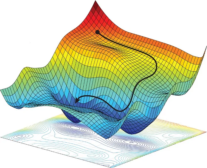
Figure: Visualization of SSE in non-linear regression. (Amini, Alexander, et al. “Spatial uncertainty sampling for end-to-end control.” arXiv preprint arXiv:1805.04829 (2018).)
Challenges in Non-Linear Compared to Linear Regression
Linear Regression:
Minimizes SSE by solving the normal equations.
\[ \boldsymbol{\beta} = (\mathbf{X}^\top \mathbf{X})^{-1} \mathbf{X}^\top \mathbf{y} \]
Closed-form solution: Direct computation of parameters without iteration.
Closed-form means the solution can be expressed explicitly using a finite number of standard mathematical operations.
Example:
Given data points \((x_i, y_i)\), calculate \(\beta_0\) and \(\beta_1\) in \(y = \beta_0 + \beta_1 x\) analytically.
Non-linear Regression:
SSE leads to non-linear equations in \(\boldsymbol{\beta}\).
\[ \boldsymbol{\beta} = \text{argmin}_{\boldsymbol{\beta}} \sum_{i=1}^{n} [ y_i - f(x_i, \boldsymbol{\beta}) ]^2 \]
No closed-form solution is available.
Parameters must be estimated using iterative optimization methods.
No closed-form solution means we cannot solve for \(\boldsymbol{\beta}\) explicitly and must use numerical methods.
Example:
Fitting \( y = \beta_0 e^{\beta_1 x} \) requires iterative algorithms like Gauss-Newton or Levenberg-Marquardt.
Using the Taylor Series Expansion for Optimization
Why use the Taylor Series?
To approximate how changes in parameters \(\boldsymbol{\beta}\) affect the model predictions \(f(x_i, \boldsymbol{\beta})\).
Helps understand how residuals and RSS change when adjusting \(\boldsymbol{\beta}\).
Allows linearization of the non-linear function around current parameter estimates.
Taylor Series Approximation:
\[ \underbrace{f(x_i, \boldsymbol{\beta})}_{\text{updated model}} \approx \underbrace{f(x_i, \boldsymbol{\beta}^{(k)})}_{\text{current model}} + \underbrace{\nabla f(x_i, \boldsymbol{\beta}^{(k)})}_{\text{change per update}} \underbrace{(\boldsymbol{\beta} - \boldsymbol{\beta}^{(k)})}_{\text{update}} \]
\(\boldsymbol{\beta}^{(k)}\): Current estimate of parameters.
\(\nabla f(x_i, \boldsymbol{\beta}^{(k)})\): Gradient (Jacobian) with respect to \(\boldsymbol{\beta}\), i.e., partial derivatives of \(f\) with respect to \(\boldsymbol{\beta}\).
Purpose:
Linearizes the model to approximate the change in residuals when \(\boldsymbol{\beta}\) is updated.
Facilitates computation of parameter updates in iterative optimization.
Identifying the Update Direction with the Jacobian Matrix
From Function Approximation to Residual Approximation:
Starting with the Taylor series expansion:
| new model = current model + gradient * update | \( f(x_i, \boldsymbol{\beta}) \approx f(x_i, \boldsymbol{\beta}^{(k)}) + \nabla f(x_i, \boldsymbol{\beta}^{(k)}) (\boldsymbol{\beta} - \boldsymbol{\beta}^{(k)}) \) |
Residuals are defined as:
| residuals = observed - predicted | \( r_i(\boldsymbol{\beta}) = y_i - f(x_i, \boldsymbol{\beta}) \) |
Substitute the approximation of new model:
| residuals = obs. - [ cur. model + gradient * update ] | \( r_i(\boldsymbol{\beta}) \approx y_i - \left[ f(x_i, \boldsymbol{\beta}^{(k)}) + \nabla f(x_i, \boldsymbol{\beta}^{(k)}) (\boldsymbol{\beta} - \boldsymbol{\beta}^{(k)}) \right] \) |
Simplify the expression:
| residuals = residuals at cur. model - gradient * update | \( r_i(\boldsymbol{\beta}) \approx \underbrace{ \left[ y_i - f(x_i, \boldsymbol{\beta}^{(k)}) \right] }_{ r_i(\boldsymbol{\beta}^{(k)}) } - \nabla f(x_i, \boldsymbol{\beta}^{(k)}) (\boldsymbol{\beta} - \boldsymbol{\beta}^{(k)}) \) |
The Central Role of the Jacobian Matrix in Parameter Updates
The Gradient as a Central Element:
\( \nabla f(x_i, \boldsymbol{\beta}^{(k)}) \) shows how changes in parameters affect model predictions.
The Jacobian matrix \(\mathbf{J}\) encapsulates all partial derivatives and can be used for \(\nabla f(x_i, \boldsymbol{\beta}^{(k)})\):
\[ J_{ij} = \frac{\partial f(x_i, \boldsymbol{\beta}^{(k)})}{\partial \beta_j} \]
Using the Jacobian to Update Parameters:
With the residual approximation:
\[ r_i(\boldsymbol{\beta}) \approx r_i(\boldsymbol{\beta}^{(k)}) - \mathbf{J}_i (\boldsymbol{\beta} - \boldsymbol{\beta}^{(k)}) \]
We aim to minimize the sum of squared residuals:
\[ \min_{\Delta \boldsymbol{\beta}} \sum_{i=1}^{n} \left[ r_i(\boldsymbol{\beta}^{(k)}) - \mathbf{J}_i \Delta \boldsymbol{\beta} \right]^2 \]
This is a linear least squares problem in \( \Delta \boldsymbol{\beta} \).
The solution gives the parameter update:
\[ \Delta \boldsymbol{\beta} = \left( \mathbf{J}^\top \mathbf{J} \right)^{-1} \mathbf{J}^\top \mathbf{r}(\boldsymbol{\beta}^{(k)}) \]
Update parameters: \[ \boldsymbol{\beta}^{(k+1)} = \boldsymbol{\beta}^{(k)} + \Delta \boldsymbol{\beta} \]
TL;DR: Non-linear Regression in a Nutshell
Non-linear regression is fundamentally similar to linear regression.
Instead of using the design matrix \( \mathbf{X} \) and observations \( \mathbf{y} \), we use the Jacobian matrix \( \mathbf{J} \) and residuals \( \mathbf{r} \).
We iteratively update parameters to minimize the residuals:
\[ \Delta \boldsymbol{\beta} = \left( \mathbf{J}^\top \mathbf{J} \right)^{-1} \mathbf{J}^\top \mathbf{r} \] \[ \boldsymbol{\beta}^{(k+1)} = \boldsymbol{\beta}^{(k)} + \Delta \boldsymbol{\beta} \]
Repeat until convergence: Each iteration recalculates coefficients, ideally reducing residuals.
The process continues until the changes in parameters or residuals are below a specified threshold.
This method leverages linear regression techniques in each iteration on the linearized model.
Example: Setting Up the Jacobian Matrix
Non-linear Function with Two Parameters:
\[ y = \beta_0 e^{\beta_1 x} \]
\( \beta_0 \) and \( \beta_1 \) are the parameters to estimate
The function is non-linear in parameters due to \( e^{\beta_1 x} \)
Compute Partial Derivatives Analytically:
\[ \frac{\partial y}{\partial \beta_0} = e^{\beta_1 x} \] \[ \frac{\partial y}{\partial \beta_1} = \beta_0 x e^{\beta_1 x} \]
Forming the Jacobian Matrix \( \mathbf{J} \):
For each observation \( x_i \):
\[ J_{i1} = \frac{\partial f(x_i, \boldsymbol{\beta})}{\partial \beta_0} = e^{\beta_1 x_i} \] \[ J_{i2} = \frac{\partial f(x_i, \boldsymbol{\beta})}{\partial \beta_1} = \beta_0 x_i e^{\beta_1 x_i} \]
The Jacobian matrix \( \mathbf{J} \) is an \( n \times 2 \) matrix.
It is used in the parameter update equation.
Numerical Computation of Partial Derivatives
When Analytical Derivatives are Difficult:
Analytical computation may be complex or infeasible
Use numerical differentiation (finite differences)
Finite Difference Approximation:
\[ \frac{\partial f(x_i, \boldsymbol{\beta})}{\partial \beta_j} \approx \frac{f(x_i, \boldsymbol{\beta} + h \mathbf{e}_j) - f(x_i, \boldsymbol{\beta})}{h} \]
\( h \): Small increment (e.g., \( h = 10^{-5} \))
\( \mathbf{e}_j \): Unit vector with 1 at position \( j \)
Example with Our Function:
Compute \( \frac{\partial y}{\partial \beta_0} \) numerically at \( \boldsymbol{\beta}^{(k)} \):
\[ \frac{\partial y}{\partial \beta_0} \approx \frac{f(x_i, \beta_0^{(k)} + h, \beta_1^{(k)}) - f(x_i, \beta_0^{(k)}, \beta_1^{(k)})}{h} \]
Similarly for \( \frac{\partial y}{\partial \beta_1} \):
\[ \frac{\partial y}{\partial \beta_1} \approx \frac{f(x_i, \beta_0^{(k)}, \beta_1^{(k)} + h) - f(x_i, \beta_0^{(k)}, \beta_1^{(k)})}{h} \]
Repeat for all observations \( x_i \) to form \( \mathbf{J} \).
Concrete Example: Calculating the Jacobian Matrix
Given Model:
\[ y = \beta_0 e^{\beta_1 x} \]
Initial parameter estimates:
\[ \beta_0^{(0)} = .9,\quad \beta_1^{(0)} = .8 \]
We have the following data:
| x_i | y_i | \( f(x_i, \boldsymbol{\beta}^{(0)}) \) | Residual \( r_i \) |
|---|---|---|---|
| 1 | 2.718 | \( 0.9 e^{0.8 \times 1} = 2.003 \) | \( 2.718 - 2.003 = 0.715 \) |
| 2 | 7.389 | \( 0.9 e^{0.8 \times 2} = 4.458 \) | \( 7.389 - 4.458 = 2.931 \) |
| 3 | 20.085 | \( 0.9 e^{0.8 \times 3} = 9.921 \) | \( 20.085 - 9.921 = 10.164 \) |
Figure: Initial model fit to data points. (red: model, blue: data)
Concrete Example: Calculating the Jacobian Matrix
Setting Up the Jacobian Matrix \( \mathbf{J} \):
Analytical derivatives:
\[ \frac{\partial y}{\partial \beta_0} = e^{\beta_1 x}, \quad \frac{\partial y}{\partial \beta_1} = \beta_0 x e^{\beta_1 x} \]
Compute Jacobian matrix at \( \boldsymbol{\beta}^{(0)} \):
| \( \frac{\partial y}{\partial \beta_0} \) | \( \frac{\partial y}{\partial \beta_1} \) | |
|---|---|---|
| i = 1 | \( .9 e^{0.8 \times 1} = 2.226 \) | \( .9 \times 1 \times 2.226 = 2.003 \) |
| i = 2 | \( .9 e^{0.8 \times 2} = 4.953 \) | \( .9 \times 2 \times 4.953 = 8.916 \) |
| i = 3 | \( .9 e^{0.8 \times 3} = 11.023 \) | \( .9 \times 3 \times 11.023 = 29.763 \) |
Jacobian matrix \( \mathbf{J} \):
\[ \mathbf{J} = \begin{bmatrix} 2.226 & 2.003 \\ 4.953 & 8.916 \\ 11.023 & 29.763 \\ \end{bmatrix} \]
Residual vector \( \mathbf{r} \):
\[ \mathbf{r} = \begin{bmatrix} 0.715 \\ 2.931 \\ 10.164 \\ \end{bmatrix} \]
Continuation: Calculating the Parameter Update
Compute \( \mathbf{J}^\top \mathbf{J} \) and \( \mathbf{J}^\top \mathbf{r} \):
\[ \mathbf{J}^\top \mathbf{J} = \begin{bmatrix} 2.226 & 4.953 & 11.023 \\ 2.003 & 8.916 & 29.763 \\ \end{bmatrix} \begin{bmatrix} 2.226 & 2.003 \\ 4.953 & 8.916 \\ 11.023 & 29.763 \\ \end{bmatrix} = \begin{bmatrix} 151.0 & 376.7 \\ 376.7 & 969.3 \\ \end{bmatrix} \]
Compute \( \mathbf{J}^\top \mathbf{r} \):
\[ \mathbf{J}^\top \mathbf{r} = \begin{bmatrix} 2.226 & 4.953 & 11.023 \\ 2.003 & 8.916 & 29.763 \\ \end{bmatrix} \begin{bmatrix} 0.715 \\ 2.931 \\ 10.164 \\ \end{bmatrix} = \mathbf{J}^\top \mathbf{r} = \begin{bmatrix} 128.2 \\ 330.1 \\ \end{bmatrix} \]
Compute the parameter update \( \Delta \boldsymbol{\beta} \):
\[ \Delta \boldsymbol{\beta} = \left( \mathbf{J}^\top \mathbf{J} \right)^{-1} \mathbf{J}^\top \mathbf{r} = \begin{bmatrix} -0.027 \\ 0.351 \\ \end{bmatrix} \]
Updated parameters:
\[ \beta_0^{(1)} = \beta_0^{(0)} + \Delta \beta_0 = 0.9 - 0.027 = 0.873 \] \[ \beta_1^{(1)} = \beta_1^{(0)} + \Delta \beta_1 = 0.8 + 0.351 = 1.151 \]
Iterating the Parameter Update
Initial Parameters Matter
Good estimates lead to quick convergence.
Poor estimates may prevent finding a solution.
Sensitivity to Starting Values
Small changes can yield different results.
Algorithms may get stuck in local minima.
Practical Implications
Choose initial parameters carefully.
Use domain knowledge for better estimates.
Estimating Uncertainties of the Coefficients
Understanding Parameter Uncertainties
In non-linear regression, estimating the uncertainties (standard errors) of the parameters is more complex than in linear regression.
Covariance Matrix Calculation
\[ \text{Cov}(\boldsymbol{\beta}) = \sigma^2 (\mathbf{J}^\top \mathbf{J})^{-1} \] where \( \sigma^2 \) is the estimated variance of the residuals.
Estimated Variance of Residuals
\[ \sigma^2 = \frac{\text{RSS}}{n - p} \] where \( \text{RSS} \) is the residual sum of squares and \( n \) is the number of observations and \( p \) is the number of parameters.
Constructing Confidence Intervals
Instead of SE of the coefficients, we can compute confidence intervals (CIs) as we cannot assume normality.
This also means that hypothesis tests are not applicable.
Estimating Uncertainties of the Coefficients
Constructing Confidence Intervals
The standard errors \( SE(\beta_j) \) are the square roots of the diagonal elements of the covariance matrix.
The \( (1 - \alpha) \times 100\% \) confidence interval for \( \beta_j \) is:
\[ \beta_j \pm z \times SE(\beta_j) \] where \( z \) is the critical value from the normal distribution, e.g., \( z = 1.96 \) for a 95% CI.
Interpreting CIs
The CI indicates the range in which the true parameter value is expected.
If the CI includes zero, the parameter is not significantly different from zero.
Non-Linear Regression: Seminar
Data Overview:
      x     y
      1.9   351.8
      2     545.0
      2.1   717.3
      2.2   947.1
      2.3   1070.8
      2.4   1048.8
      2.5   806.4
      2.6   761.7
      2.7   826.1
Task:
Fit a non-linear regression model to the data. Use the function:
\[y = a \cdot \exp\left(-0.5 \frac{(x - b)^2}{c^2}\right) + d \cdot x^2 + e\]
Estimate the parameters \(a\), \(b\), \(c\), \(d\), and \(e\).
Hint: for check-up these should be quite good parameters:
a = 600, b = 2.3, c = 0.15, d = 100, e = 20