Chemometrics & Statistics
06. Data Modeling 1Linear Regression
Imagine you have measured some data: Water quality and nutrient levels
You monitor nitrate levels and algal growth in a lake.
Nitrate concentration
  x (Nitrate) mg/L
    = [1, 2, 3, 4, 5]
Algal growth (chlorophyll-a)
  y (Algal growth) µg/L
    = [10, 20, 35, 50, 70]
Is there a trend between nutrient levels and algal growth?
Can we predict algal growth if nitrate levels increase further?
\[ y = f(x) + \varepsilon \] Can this model capture the relationship?
Where is linear regression used?
Trend analysis
Detecting changes in pollutant levels over time.
Calibration
Relating instrument response to known concentrations.
Predictive modeling
Estimating future values (e.g., water quality metrics).
Example 1:
Monitoring nitrate levels in a river over 10 years to detect trends.
Example 2:
Calibrating a spectrophotometer for phosphate detection.
Example 3:
Predicting algal bloom occurrence based on nutrient inputs.
Some important terms
Dependent variable (\(y\))
The value we explain or predict.
Independent variable (\(x\))
The input or predictor variable(s).
Error term (\(\varepsilon\))
The difference between observed and predicted \(y\).
Coefficients (\(\beta_0, \beta_1, \dots \beta_n\))
Intercept, slope, quadratic terms, etc. These describe the layout of the regression line.
Estimates \(y\) \(\hat{y}\), \(\beta\) \(\hat{\beta}\)
Predicted value based on the regression model and estimated coefficients. The hat symbol denotes estimates.
Uncertainties \(\sigma^2\), \(s^2\)
How confident are we in the model? How precise are the coefficients?
Some important terms cont,
Squared error term (\(SSE\))
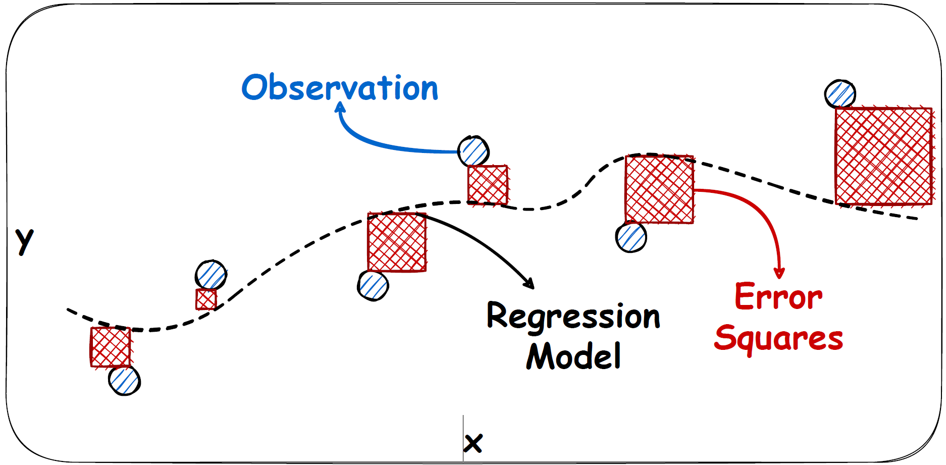
Basic principle of linear regression
Linear Model Definition:
\[ y = \sum\left(\beta_i x_i\right) + \varepsilon = \hat{y} + \varepsilon \]
Strategy:
Find coefficients \(\beta_i\) that minimize the error term \(\varepsilon\).
Error: Difference between observed \(y\) and predicted \(\hat{y}\).
Objective:
Minimize the sum of squared errors (SSE): \[ \text{SSE} = \sum (y_i - \hat{y}_i)^2 \]
Mathematical background
Strategy:
Minimize the Sum of Squared Errors (SSE):
\[
\text{SSE} = \sum_{i=1}^n \left(y_i - (\beta_0 + \beta_1 x_i)\right)^2
\]
where \(n\) is the number of data points, \(y_i\) is the observed value, \(x_i\) is the predictor, and \(\beta_i\) are the coefficients.
How to find the minimum:
Take the derivative of SSE with respect to \(\beta_0\) and \(\beta_1\).
Solve the resulting equations for \(\beta_0\) and \(\beta_1\).
Derivative with respect to \(\beta_1\):
\[
\frac{\partial \text{SSE}}{\partial \beta_1} = -2 \sum_{i=1}^n x_i \left(y_i - (\beta_0 + \beta_1
x_i)\right)
\]
Derivative with respect to \(\beta_0\):
\[
\frac{\partial \text{SSE}}{\partial \beta_0} = -2 \sum_{i=1}^n \left(y_i - (\beta_0 + \beta_1 x_i)\right)
\]
Setting both derivatives to zero gives equations for \(\beta_0\) and \(\beta_1\).
Instead of solving these equations by hand, we can use matrix operations.
Some words on matrix operations
What is a matrix?
A rectangular array of numbers arranged in rows and columns:
\[
\mathbf{A} = \begin{bmatrix}
a_{11} & a_{12} & \cdots & a_{1n} \\
a_{21} & a_{22} & \cdots & a_{2n} \\
\vdots & \vdots & \ddots & \vdots \\
a_{m1} & a_{m2} & \cdots & a_{mn}
\end{bmatrix}
\]
\(m\): Number of rows.
\(n\): Number of columns.
A matrix is often denoted by a bold uppercase letter.
Key matrix operations:
Transpose: Flips rows and columns.
\[
\mathbf{A}^\top = \begin{bmatrix}
a_{11} & a_{21} & \cdots & a_{m1} \\
a_{12} & a_{22} & \cdots & a_{m2} \\
\vdots & \vdots & \ddots & \vdots \\
a_{1n} & a_{2n} & \cdots & a_{mn}
\end{bmatrix}
\]
an (n x m) matrix becomes an (m x n) matrix.
Transpose is denoted by a superscript T or a prime symbol, e.g., \(\mathbf{A}^T\) or \(\mathbf{A}'\).
continue on next slide.
Some words on matrix operations cont,
Adding or subtracting matrices: \[ \mathbf{A} + \mathbf{B} = \begin{bmatrix} a_{11} & a_{12} \\ a_{21} & a_{22} \end{bmatrix} + \begin{bmatrix} b_{11} & b_{12} \\ b_{21} & b_{22} \end{bmatrix} = \begin{bmatrix} a_{11} + b_{11} & a_{12} + b_{12} \\ a_{21} + b_{21} & a_{22} + b_{22} \end{bmatrix} \]
Every element of the first matrix is added to the corresponding element of the second matrix.
The resulting matrix has the same number of rows and columns as the original matrices.
Therefore, it requires that both matrices have the same number of rows and columns.
Some words on matrix operations cont,
Multiplying matrices: \[ \mathbf{A} = \begin{bmatrix} 1 & 2 \\ 3 & 4 \end{bmatrix}, \quad \mathbf{B} = \begin{bmatrix} 5 & 6 \\ 7 & 8 \end{bmatrix} \] \[ \mathbf{C} = \mathbf{A} \cdot \mathbf{B} = \begin{bmatrix} 1 \cdot 5 + 2 \cdot 7 & 1 \cdot 6 + 2 \cdot 8 \\ 3 \cdot 5 + 4 \cdot 7 & 3 \cdot 6 + 4 \cdot 8 \end{bmatrix} = \begin{bmatrix} 19 & 22 \\ 43 & 50 \end{bmatrix} \]
Every element of a row in the first matrix is multiplied by every element of a column in the second matrix.
The resulting matrix has the same number of rows as the first matrix and the same number of columns as the second matrix, i.e., (m x p) * (p x n) = (m x n).
Therefore, it requires that the number of columns in the first matrix equals the number of rows in the second matrix.
Some words on matrix operations cont,
Inverting a matrix: \[ \mathbf{A} = \begin{bmatrix} a & b \\ c & d \end{bmatrix}, \quad \mathbf{A}^{-1} = \frac{1}{ad - bc} \begin{bmatrix} d & -b \\ -c & a \end{bmatrix} \]
The inverse of a matrix is a matrix that, when multiplied with the original matrix, results in the identity matrix. \( \mathbf{A} \cdot \mathbf{A}^{-1} = \mathbf{I} \).
The identity matrix is a square matrix with ones on the diagonal and zeros elsewhere.
The inverse of a matrix is denoted by a superscript -1, e.g., \(\mathbf{A}^{-1}\).
It is the analog of a division.
Using matrices to minimize SSE
Regression equation:
In scalar form:
\[
y_i = \beta_0 + \beta_1 x_{i1} + \ldots + \beta_p x_{ip} + \varepsilon_i
\]
In matrix form:
\[
\mathbf{y} = \mathbf{X} \mathbf{\beta} + \mathbf{\varepsilon}
\]
where \(\mathbf{y}\) is the vector of observed values, \(\mathbf{X}\) is the matrix of predictors, and
\(\mathbf{\beta}\) is the vector of coefficients.
Objective:
Minimize the Sum of Squared Errors (SSE):
\[
\text{SSE} = \|\mathbf{y} - \mathbf{X} \mathbf{\beta}\|^2
\]
The \(\|\cdot\|^2\) denotes the squared Euclidean norm and is equivalent to: \[\underbrace{(\mathbf{y} - \mathbf{X} \mathbf{\beta})^\top}_{\varepsilon^\top} \underbrace{(\mathbf{y} - \mathbf{X} \mathbf{\beta})}_{\varepsilon}\]
e.g., \[ \begin{bmatrix} 1 \\ 2 \\ 3 \end{bmatrix}^\top \begin{bmatrix} 1 \\ 2 \\ 3 \end{bmatrix} = \begin{bmatrix} 1 & 2 & 3 \end{bmatrix} \begin{bmatrix} 1 \\ 2 \\ 3 \end{bmatrix} = 1 \cdot 1 + 2 \cdot 2 + 3 \cdot 3 = 14 \]
Deriving the Normal Equation
Start with SSE:
The objective is to minimize the Sum of Squared Errors (SSE): \[ \text{SSE} = (\mathbf{y} - \mathbf{X} \mathbf{\beta})^\top (\mathbf{y} - \mathbf{X} \mathbf{\beta}) \]
Expand SSE:
Expand the quadratic form:
\[ \text{SSE} = \mathbf{y}^\top \mathbf{y} - 2 \mathbf{\beta}^\top \mathbf{X}^\top \mathbf{y} + \mathbf{\beta}^\top \mathbf{X}^\top \mathbf{X} \mathbf{\beta} \]
Derivative with respect to \(\mathbf{\beta}\):
Take the derivative to find the minimum:
\[
\frac{\partial \text{SSE}}{\partial \mathbf{\beta}} = -2 \mathbf{X}^\top \mathbf{y} + 2 \mathbf{X}^\top
\mathbf{X} \mathbf{\beta}.
\]
Set derivative to zero:
Solve for \(\mathbf{\beta}\):
\[
-2 \mathbf{X}^\top \mathbf{y} + 2 \mathbf{X}^\top \mathbf{X} \mathbf{\beta} = 0
\]
Simplify:
\[
\mathbf{X}^\top \mathbf{X} \mathbf{\beta} = \mathbf{X}^\top \mathbf{y}
\]
Solution (Normal Equation):
Multiply by the inverse of \(\mathbf{X}^\top \mathbf{X}\):
\[
\mathbf{\hat{\beta}} = (\mathbf{X}^\top \mathbf{X})^{-1} \mathbf{X}^\top \mathbf{y}
\]
This gives the least-squares solution for \(\mathbf{\beta}\).
Example
Data setup:
Observations (\(n = 4\))
Predictors x = [1, 2, 3, 4]
Response y = [3, 6, 8, 11]
Coefficients: b0, b1, b2 , i.e., intercept, slope, quadratic term.
The selection of coefficients sets up the model layout and depends on the data.
Set up the Design matrix (\(\mathbf{X}\)):
Based on the predictors \(x\) and the model layout, we set up the matrix like: \[ \mathbf{X} = \begin{bmatrix} x_1^0 & x_1^1 & x_1^2 \\ x_2^0 & x_2^1 & x_2^2 \\ \vdots & \vdots & \vdots \\ x_n^0 & x_n^1 & x_n^2 \end{bmatrix} = \begin{bmatrix} 1 & 1 & 1 \\ 1 & 2 & 4 \\ 1 & 3 & 9 \\ 1 & 4 & 16 \end{bmatrix} \]
The columns represent the predictors and their powers, e.g., first colum is the intercept, so x to the power of 0, second column is the linear term, so x to the power of 1, and so on.
Example cont,
Step 1: Compute \(\mathbf{X}^\top \mathbf{X}\)
A) Recall the Design matrix: \[ \mathbf{X} = \begin{bmatrix} 1 & 1 & 1 \\ 1 & 2 & 4 \\ 1 & 3 & 9 \\ 1 & 4 & 16 \end{bmatrix} \]
B) Transpose of \(\mathbf{X}\): \[ \mathbf{X}^\top = \begin{bmatrix} 1 & 1 & 1 & 1 \\ 1 & 2 & 3 & 4 \\ 1 & 4 & 9 & 16 \end{bmatrix} \]
C) Multiply \(\mathbf{X}^\top \mathbf{X}\): \[ \mathbf{X}^\top \mathbf{X} = \begin{bmatrix} 1 & 1 & 1 & 1 \\ 1 & 2 & 3 & 4 \\ 1 & 4 & 9 & 16 \end{bmatrix} \begin{bmatrix} 1 & 1 & 1 \\ 1 & 2 & 4 \\ 1 & 3 & 9 \\ 1 & 4 & 16 \end{bmatrix} = \begin{bmatrix} 4 & 10 & 30 \\ 10 & 30 & 100 \\ 30 & 100 & 354 \end{bmatrix} \]
Example cont.
Step 3: Compute \((\mathbf{X}^\top \mathbf{X})^{-1}\)
A) Recall \(\mathbf{X}^\top \mathbf{X}\): \[ \mathbf{X}^\top \mathbf{X} = \begin{bmatrix} 4 & 10 & 30 \\ 10 & 30 & 100 \\ 30 & 100 & 354 \end{bmatrix} \] The matrix is symmetric and positive-definite, so it is invertible.
B) Inverse of \(\mathbf{X}^\top \mathbf{X}\): \[ (\mathbf{X}^\top \mathbf{X})^{-1} = \begin{bmatrix} 7.75 & -6.75 & 1.25 \\ -6.75 & 6.45 & -1.25 \\ 1.25 & -1.25 & 0.25 \end{bmatrix} \]
Why is this important?
\((\mathbf{X}^\top \mathbf{X})^{-1}\) is crucial for calculating the coefficients \(\mathbf{\beta}\):
\[
\mathbf{\hat{\beta}} = (\mathbf{X}^\top \mathbf{X})^{-1} \mathbf{X}^\top \mathbf{y}.
\]
It also provides information about the variance-covariance structure of \(\mathbf{\beta}\).
Example cont.
Step 4: Compute the Pseudo-Inverse of \(\mathbf{X}\)
The pseudo-inverse of \(\mathbf{X}\) is defined as: \[ \mathbf{X}^+ = (\mathbf{X}^\top \mathbf{X})^{-1} \mathbf{X}^\top \]
Multiply \((\mathbf{X}^\top \mathbf{X})^{-1} \mathbf{X}^\top\): \[ \mathbf{X}^+ = \begin{bmatrix} 7.8 & -6.8 & 1.3 \\ -6.8 & 6.5 & -1.3 \\ 1.3 & -1.3 & 0.3 \end{bmatrix} \begin{bmatrix} 1 & 1 & 1 & 1 \\ 1 & 2 & 3 & 4 \\ 1 & 4 & 9 & 16 \end{bmatrix} = \begin{bmatrix} 2.3 & -0.8 & -0.3 & 0.8 \\ -1.6 & 1.2 & 1.4 & -1.0 \\ 0.3 & -0.3 & -0.3 & 0.3 \end{bmatrix} \]
Example cont.
Step 5: Calculate \(\mathbf{\hat{\beta}}\) (the coefficients)
The coefficients are calculated using the pseudo-inverse: \[ \mathbf{\hat{\beta}} = \mathbf{X}^+ \mathbf{y} \]
Recall: \[ \mathbf{X}^+ = \begin{bmatrix} 2.3 & -0.8 & -0.3 & 0.8 \\ -1.6 & 1.2 & 1.4 & -1.0 \\ 0.3 & -0.3 & -0.3 & 0.3 \end{bmatrix} \] \[ \mathbf{y} = \begin{bmatrix} 3 \\ 6 \\ 8 \\ 11 \end{bmatrix} \]
Multiply \(\mathbf{X}^+\) and \(\mathbf{y}\): \[ \mathbf{\hat{\beta}} = \begin{bmatrix} 0.5 \\ 2.6 \\ 0.0 \end{bmatrix} \]
Interpretation:
The estimated coefficients are:
\(b_0 = 0.5\): Intercept (baseline \(x = 0\)).
\(b_1 = 2.6\): Linear slope of \(x\).
\(b_2 = 0.0\): Quadratic effect of \(x^2\).
Example cont.
Visualizing the Model
The estimated coefficients: \[ \mathbf{\hat{\beta}} = \begin{bmatrix} 0.5 \\ 2.6 \\ 0.0 \end{bmatrix} \] The equation of the fitted model: \[ y = 0.5 + 2.6x + 0.0x^2 \]
Uncertainties in Linear Regressions
Variance of \(y\) (\(\sigma^2\)):
The total variance in the observed data (\(y\)) is denoted by \(\sigma^2\).
It measures the spread of the actual \(y\)-values around the fitted model (\(\hat{y}\)): \[ \sigma^2 = \frac{\sum (y_i - \hat{y}_i)^2}{n - p - 1} \]
where \(n\) is the number of observations and \(p\) is the number of coefficients excluding the intercept.
This is also called the residual variance or mean squared error (MSE).
Key Insights:
Higher variance in \(y\) leads to higher uncertainty in the predictions.
A poorly fitted model will have larger residuals, increasing \(\sigma^2\).
Variance of \(\beta\) (\(\sigma^2_\beta\)):
The coefficients \(\beta\) are also estimated with uncertainty, which depends on:
The residual variance (\(\sigma^2\)).
The structure of the predictor matrix (\(\mathbf{X}\)).
Uncertainties of Coefficients: Introduction
Ideal Case: Multiple Measurement Series
If we had multiple measurement series (\(k\)) with the same predictors, we could estimate multiple sets of coefficients \(\mathbf{\beta}_1, \mathbf{\beta}_2, \ldots, \mathbf{\beta}_k\).
By analyzing the variability between these sets, we could directly calculate the variances and covariances of the coefficients: \[ \text{Var}(\beta_i) = \frac{1}{k} \sum_{j=1}^k (\beta_{i,j} - \overline{\beta}_i)^2 \]
I.e., the variance of the intercept (\(\beta_0\)) would be the average squared difference between the intercepts of the different sets.
The Problem:
In practice, we often only have one measurement series, which means:
We cannot directly calculate the variability of \(\beta\) from multiple sets.
Uncertainties of Coefficients: Derivation
Start from the Model:
The linear regression model is: \[ \mathbf{y} = \mathbf{X} \mathbf{\beta} + \mathbf{\varepsilon} \]
The OLS estimator for \(\mathbf{\beta}\) is: \[ \mathbf{\hat{\beta}} = (\mathbf{X}^\top \mathbf{X})^{-1} \mathbf{X}^\top \mathbf{y} \]
Deriving \(\text{Var}(\mathbf{\beta})\):
Substitute \(\mathbf{y} = \mathbf{X} \mathbf{\beta} + \mathbf{\varepsilon}\) into \(\mathbf{\hat{\beta}}\): \[ \mathbf{\hat{\beta}} = (\mathbf{X}^\top \mathbf{X})^{-1} \mathbf{X}^\top (\mathbf{X} \mathbf{\beta} + \mathbf{\varepsilon}) \]
Expand: \[ \mathbf{\hat{\beta}} = \mathbf{\beta} + (\mathbf{X}^\top \mathbf{X})^{-1} \mathbf{X}^\top \mathbf{\varepsilon} \]
Take the variance (\(\text{Var}(\beta)=0\)): \[ \text{Var}(\mathbf{\hat{\beta}}) = \text{Var}((\mathbf{X}^\top \mathbf{X})^{-1} \mathbf{X}^\top \mathbf{\varepsilon}) \]
Since \((\mathbf{X}^\top \mathbf{X})^{-1} \mathbf{X}^\top\) is a constant, we can pull it out like: \(\text{Var}(\mathbf{A}\varepsilon) = \mathbf{A} \text{Var}(\varepsilon) \mathbf{A}^\top\) and get:
\[ \text{Var}(\mathbf{\hat{\beta}}) = \underbrace{(\mathbf{X}^\top \mathbf{X})^{-1} \mathbf{X}^\top}_{\mathbf{A}} \text{Var}(\varepsilon) \underbrace{\left((\mathbf{X}^\top \mathbf{X})^{-1} \mathbf{X}^\top\right)^\top}_{\mathbf{A}^\top} \]
This can be simplified to:
\[ \text{Var}(\mathbf{\hat{\beta}}) = (\mathbf{X}^\top \mathbf{X})^{-1} \mathbf{X}^\top \text{Var}(\varepsilon) \mathbf{X} (\mathbf{X}^\top \mathbf{X})^{-1} \]
Uncertainties of Coefficients: Derivation cont.
Recall:
\[ \text{Var}(\mathbf{\hat{\beta}}) = (\mathbf{X}^\top \mathbf{X})^{-1} \mathbf{X}^\top \text{Var}(\varepsilon) \mathbf{X} (\mathbf{X}^\top \mathbf{X})^{-1} \]
To solve this we apply the Gauss-Markov theorem. \[ \text{Var}(\varepsilon) = \sigma^2 \] i.e., the variance of the residuals is a homoscedastic constant (scalar) that can be moved within the equation.
Move the variance... \[ \text{Var}(\mathbf{\hat{\beta}}) = \sigma^2 (\mathbf{X}^\top \mathbf{X})^{-1} \underbrace{\mathbf{X}^\top \mathbf{X} (\mathbf{X}^\top \mathbf{X})^{-1}}_{A \cdot A^{-1} = 1} \]
...and the terms collapse:
\[ \text{Var}(\mathbf{\hat{\beta}}) = \sigma^2 (\mathbf{X}^\top \mathbf{X})^{-1} \]
Variance-Covariance Matrix: Example
Data Overview:
Observed values (\(y\)) and predicted values (\(\hat{y}\)) based on the model:
x = [1, 2, 3, 4]
y = [3, 6, 8, 11]
y_hat = [3.1, 5.7, 8.3, 10.9]
Residual variance (\(\text{MSE}\)):
mse = 0.2
Inverse of \(\mathbf{X}^\top \mathbf{X}\):
\[ (\mathbf{X}^\top \mathbf{X})^{-1} = \begin{bmatrix} 7.75 & -6.75 & 1.25 \\ -6.75 & 6.45 & -1.25 \\ 1.25 & -1.25 & 0.25 \end{bmatrix} \]
Calculating the Variance-Covariance Matrix:
Using the formula: \[ \text{Var}(\mathbf{\hat{\beta}}) = \sigma^2 (\mathbf{X}^\top \mathbf{X})^{-1}, \] we compute: \[ \text{Var}(\mathbf{\hat{\beta}}) = 0.2 \cdot \begin{bmatrix} 7.75 & -6.75 & 1.25 \\ -6.75 & 6.45 & -1.25 \\ 1.25 & -1.25 & 0.25 \end{bmatrix} \]
Result: \[ \text{Var}(\mathbf{\hat{\beta}}) = \begin{bmatrix} 1.55 & -1.35 & 0.25 \\ -1.35 & 1.29 & -0.25 \\ 0.25 & -0.25 & 0.05 \end{bmatrix} \]
Significance of Coefficients
Using the Variance-Covariance Matrix:
From the variance-covariance matrix \(\text{Var}(\mathbf{\hat{\beta}})\), we can derive:
Standard Error (SE) of each coefficient (\(b_i\)): \[ \text{SE}(b_i) = \sqrt{\text{diag}(\text{Var}(\mathbf{\hat{\beta}}))} \]
t-statistic for each coefficient: \[ t_i = \frac{b_i}{\text{SE}(b_i)} \]
These values allow us to test the null hypothesis: \[ H_0: b_i = 0 \quad \text{(no effect)}. \] \[ H_1: b_i \neq 0 \quad \text{(significant effect)}. \]
Interpreting the Results:
Compare the \(t_i\)-statistic to the critical value from the t-distribution:
Degrees of freedom: \(n - p - 1\) (number of observations minus number of predictors and intercept).
If \(|t_i| > t_{\text{critical}}\), the coefficient is significant, i.e., it has a statistically significant effect.
Example: Significance Testing of Coefficients
Coefficients and Standard Errors:
From the regression model, we have:
b0 = 0.5, b1 = 2.6, b2 = 0.0
Calculated standard errors:
SE(b0) = sqrt(1.55) = 1.24
SE(b1) = sqrt(1.29) = 1.14
SE(b2) = sqrt(0.05) = 0.22
Calculate t-statistics:
t0 =  0.5 / 1.24 = 0.40
t1 = 2.6 / 1.14 = 2.28
t2 = 0.0 / 0.22 = 0.00
Interpreting the Results:
Degrees of freedom:
\(n - p - 1 = 4 - 2 - 1 = 1\).
Critical value for \(t_{\text{critical}}\) at \(\alpha = 0.05\) (two-tailed): \(\pm 12.71\).
\(t_0 = 0.40\): Not significant
\(t_1 = 2.28\): Not significant
\(t_2 = 0.00\): Not significant
Conclusion:
Model not suitable, remove coefficient with worst t-statistic and re-evaluate.
Recalculated Model Results
New Model:
After excluding \(b_2\) (quadratic term), the design matrix becomes:
\[ \mathbf{X} = \begin{bmatrix} 1 & 1 \\ 1 & 2 \\ 1 & 3 \\ 1 & 4 \end{bmatrix} \quad \text{and} \quad \mathbf{X}^\top \mathbf{X} = \begin{bmatrix} 4 & 10 \\ 10 & 30 \end{bmatrix} \]
The inverse of \(\mathbf{X}^\top \mathbf{X}\):
\[ (\mathbf{X}^\top \mathbf{X})^{-1} = \begin{bmatrix} 1.5 & -0.5 \\ -0.5 & 0.2 \end{bmatrix} \]
New coefficients: \[ \mathbf{\hat{\beta}} = \begin{bmatrix} 0.5 \\ 2.6 \end{bmatrix} \]
Variance-Covariance Matrix:
The recalculated variance-covariance matrix: \[ \text{Var}(\mathbf{\hat{\beta}}) = \begin{bmatrix} 0.3 & -0.1 \\ -0.1 & 0.04 \end{bmatrix}. \]
Significance of Coefficients:
t-statistics:
t0 = 0.5 / 0.55 = 0.91
t1 = 2.6 / 0.2 = 13.00
\(t_1\) is highly significant (\(t_1 > t_{\text{critical}}\)), confirming the importance of \(x_1\).
The intercept \(b_0\) should not be removed even though it is not significant.
Global F-Test in Linear Regression
Purpose:
Test whether the entire regression model is significant.
Null hypothesis (\(H_0\)):
All coefficients except the intercept are 0
(\(\beta_1 = \beta_2 = \ldots = \beta_p = 0\)).
Alternative hypothesis (\(H_1\)): At least one coefficient is not zero.
F-statistic Formula:
\[ F = \frac{\text{SSR} / p}{\text{SSE} / (n - p - 1)} \] where \(p\) is the number of predictors and \(n\) is the number of observations.
Thereby, \[ \text{SSR} = \sum (\hat{y}_i - \overline{y})^2 \quad \text{and} \quad \text{SSE} = \sum (y_i - \hat{y}_i)^2 \]
Interpreting the F-statistic:
Compare \(F\) to the critical value from the F-distribution:
Degrees of freedom: \(p\) (numerator) and \(n - p - 1\) (denominator).
If \(F > F_{\text{critical}}\), reject \(H_0\): The model is significant.
Quality Metrics for Regression
Evaluating the Regression Model:
\(R^2\) (Coefficient of Determination):
\[ R^2 = 1 - \frac{\text{SSE}}{\text{SST}} \] Measures the proportion of variance in \(y\) explained by the model. Ranges from 0 to 1. \(\text{SST}\) is the total sum of squares and \(\text{SSE}\) is the sum of squared errors.
Adjusted \(R^2\):
\[ R^2_{\text{adj}} = 1 - \frac{\text{SSE}/(n - p - 1)}{\text{SST}/(n - 1)} \] Adjusts \(R^2\) for the number of predictors. Useful when comparing models with different numbers of predictors.
RMSE (Root Mean Squared Error):
\[ \text{RMSE} = \sqrt{\frac{\text{SSE}}{n - p - 1}} \] Measures the average error of the model in predicting \(y\).
Other Useful Metrics:
MAE (Mean Absolute Error):
\[ \text{MAE} = \frac{\sum_{i=1}^n |y_i - \hat{y}_i|}{n} \] Measures the average absolute difference between observed and predicted values.
Confidence in Linear Regressions
What is a Confidence Interval (CI)?
A confidence interval estimates the range in which the true population parameter (e.g., coefficient) is likely to lie with a specified level of confidence (e.g., 95%).
CI for Fitted Values (\(\hat{y}\)):
For a given predictor vector \(\mathbf{x}\), the confidence interval of the fitted value is: \[ \text{CI}(\hat{y}) = \hat{y} \pm t_{\text{critical}} \cdot \sqrt{\mathbf{x}^\top \text{Var}(\mathbf{\hat{\beta}}) \mathbf{x}} \] where \(\text{Var}(\mathbf{\hat{\beta}})\) is the variance-covariance matrix of the coefficients and \(\mathbf{x}\) is the predictor vector (not the design matrix). I.e., for \(x = 3\): \(\mathbf{x} = [1, 3]\).
Predictions in Linear Regressions
What is a Prediction Interval (PI)?
A prediction interval estimates the range in which a new observation (\(y_{\text{new}}\)) is likely to fall, given the model.
Formula for Prediction Interval:
For a given predictor vector \(\mathbf{x}\), the prediction interval is: \[ \text{PI}(y_{\text{new}}) = \hat{y} \pm t_{\text{critical}} \cdot \sqrt{\mathbf{x}^\top \text{Var}(\mathbf{\hat{\beta}}) \mathbf{x} + \sigma^2} \]
where \(\sigma^2\) is the residual variance (MSE) and \(\text{Var}(\mathbf{\hat{\beta}})\) is the variance-covariance matrix of the coefficients.
Key Differences Between CI and PI:
Confidence Intervals: Uncertainty about the mean response (\(\hat{y}\)).
Prediction Intervals: Uncertainty about a new observation (\(y_{\text{new}}\)).
PI includes both the variability in \(\hat{y}\) and the residual variance (\(\sigma^2\)).
Example
Linear Regression: Seminar
Data Overview:
      x     y
      0     5.9968
      2.5   10.2135
      5     13.3713
      7.5   18.6136
      10    18.5819
Task:
Fit a linear regression model to the data.
Calculate the Confidence Interval (CI) for the regression line.
Calculate the Prediction Interval (PI) for new observations.