Chemometrics & Statistics
05. Similarity Analysis 3Mulitvariate Similarity Analysis
Initial thoughts on multivariate data analysis
Let's assume we have a data set that contains the following information:
Each sample was measured with 10 replicates and the mean values are given in the table below.
                  ┌────────┬───────┐
                  │ Sample │ [Fe]  │
                  ├────────┼───────┤
                  │    1   │  2.3  │
                  │    2   │  2.7  │
                  │    3   │  1.9  │
                  │    4   │  2.1  │
                  │    5   │  2.5  │
                  └────────┴───────┘
We already know how to compare these samples, e.g., using ANOVA or t-test.
Initial thoughts on multivariate data analysis
Now, let's assume we have a data set that contains the following information:
Each sample was measured with 10 replicates and the mean values are given in the table below.
                  ┌────────┬───────┬───────┬───────┬───────┐
                  │ Sample │ [Fe]  │ [Cu]  │ [Zn]  │ [Mn]  │
                  ├────────┼───────┼───────┼───────┼───────┤
                  │    1   │  2.3  │  1.2  │  0.5  │  0.2  │
                  │    2   │  2.7  │  1.1  │  0.4  │  0.3  │
                  │    3   │  1.9  │  1.3  │  0.6  │  0.1  │
                  │    4   │  2.1  │  1.0  │  0.3  │  0.4  │
                  │    5   │  2.5  │  1.4  │  0.7  │  0.5  │
                  └────────┴───────┴───────┴───────┴───────┘
How can we compare these samples?
Similarity Measures - Metrics
There are several metrics available to calculate the similarity between samples with multiple variables (multivariate data).
Minkowski distance is a generalization of distances and is defined as:
\[ d = \left( \sum_{i=1}^{n} |x_i - y_i|^p \right)^{1/p} \]
Where \(x_i\) and \(y_i\) are the values of the \(i\)-th variable of the samples \(x\) and \(y\),
respectively.
Manhattan distance (L1 norm) is defined as:
\[ d = \sum_{i=1}^{n} |x_i - y_i| \]
Where \(x_i\) and \(y_i\) are the values of the \(i\)-th variable of the samples \(x\) and \(y\),
respectively.
Euclidean distance (L2 norm) is defined as:
\[ d = \sqrt{\sum_{i=1}^{n} (x_i - y_i)^2} \]
Where \(x_i\) and \(y_i\) are the values of the \(i\)-th variable of the samples \(x\) and \(y\),
respectively.
Minkowski Distance
The Minkowski distance is a generalized difference-based metric: \[ d = \left( \sum_{i=1}^{n} |x_i - y_i|^p \right)^{1/p} \] where \( p \) is the order of the distance. Adjust \( p \) with the slider to see how the distance calculation changes.
Example: given the following data points:
                A = [5.2, 3.9, 2.1, 1.8, 0.7]
                B = [4.8, 3.7, 2.0, 1.7, 0.6]
                  d = |5.2 - 4.8|^1 + |3.9 - 3.7|^1
                    + |2.1 - 2.0|^1 + |1.8 - 1.7|^1
                    + |0.7 - 0.6|^1

                  d = 0.40 + 0.20 + 0.10 + 0.10 + 0.10

                  d = 0.90
Correlation-based Similarity Measures
Correlation coefficients quantify the similarity between variables by measuring linear relationships.
Pearson Correlation: Measures linear relationships between two variables, ranging from -1 to
+1.
\[
r = \frac{\sum (x_i - \bar{x})(y_i - \bar{y})}{\sqrt{\sum (x_i - \bar{x})^2 \sum (y_i - \bar{y})^2}}
\]
where \(\bar{x}\) and \(\bar{y}\) are the means of the variables.
\[d = 1 - r\] where \(r\) is the Pearson correlation coefficient and \(d\) is the distance.
Example: given the following data points:
                A = [5.2, 3.9, 2.1, 1.8, 0.7]
                B = [4.8, 3.7, 1.8, 1.9, 0.6]
                  A_mean = 2.94
                  B_mean = 2.56

                  Cov(A, B) = 1 / (N-1) *
                    [
                        (5.2 - 2.94) * (4.8 - 2.56)
                      + (3.9 - 2.94) * (3.7 - 2.56)
                      + (2.1 - 2.94) * (1.8 - 2.56)
                      + (1.8 - 2.94) * (1.9 - 2.56)
                      + (0.7 - 2.94) * (0.6 - 2.56)
                    ]

                  Cov(A, B) / (std(A) * std(B)) = 0.99
                  >> d = 1 - 0.99 = 0.01
Correlation-based Similarity Measures
Correlation coefficients quantify the similarity between variables by measuring linear relationships.
Spearman Correlation: Ranks* data to assess monotonic relationships, useful for non-linear
data.
\[
r_s = 1 - \frac{6 \sum d_i^2}{n(n^2 - 1)}
\]
where \(d_i\) is the difference between ranks*.
\[d = 1 - r_s\] where \(r_s\) is the Spearman correlation coefficient and \(d\) is the distance.
Example: given the following data points:
                A = [5.2, 3.9, 2.1, 1.8, 0.7]
                B = [4.8, 3.7, 1.8, 1.9, 0.6]
                  A_rank = [5, 4, 3, 2, 1]
                  B_rank = [5, 4, 1, 2, 3]

                  d = [0, 0, 2, 0, 2]

                  r_s = 1 - 6 *
                    (0^2 + 0^2 + 2^2 + 0^2 + 2^2) /
                    (5 * (5^2 - 1))

                  r_s = 0.6

                  >> d = 1 - 0.6 = 0.4
*Ranks are the position of the data in a sorted list.
Cosine Similarity as a Similarity Measure
Cosine similarity measures the similarity between two vectors by comparing their direction, normalized by their magnitudes.
Cosine Similarity: Defined as the dot product of two vectors divided by the product of their
norms.
\[
\text{similarity} = \frac{\sum_{i=1}^{n} x_i \cdot y_i}{||X|| \cdot ||Y||}
\]
where \( ||X|| = \sqrt{\sum_{i=1}^{n} x_i^2} \) and \( ||Y|| = \sqrt{\sum_{i=1}^{n} y_i^2} \).
Example: given the following vectors:
                X = [2, 3, 4]
                Y = [1, 0, 5]
                  dot_product = 2*1 + 3*0 + 4*5 = 22
                  ||X|| = sqrt(2^2 + 3^2 + 4^2) = 5.39
                  ||Y|| = sqrt(1^2 + 0^2 + 5^2) = 5.10

                  similarity = 22 / (5.39 * 5.10)

                  similarity ≈ 0.80
The cosine similarity ranges from -1 to 1, with higher values indicating greater similarity in direction.
Overview: Choosing the Right Similarity Measure
Minkowski Distance
General distance metric for multivariate data.
Adjustable: Manhattan (p=1), Euclidean (p=2).
Works best with continuous numeric data.
Pearson Correlation
Measures linear relationships.
Good for continuous, normally distributed data.
Sensitive to outliers.
Spearman Correlation
For monotonic (ranked) relationships.
Works with ordinal or non-linear data.
Less sensitive to outliers than Pearson.
Cosine Similarity
Measures similarity in vector direction.
Useful in high-dimensional data (e.g., text).
Focuses on orientation, not magnitude.
There is no one-size-fits-all similarity measure. Choose the one that best fits your data and research question.
Hierarchical Cluster Analysis (HCA)
HCA groups similar items into clusters based on their similarity or distance.
The result is a dendrogram, a tree-like structure showing the nested clusters.
Types of HCA:
Agglomerative (bottom-up): Starts with individual items and merges them into clusters.
Divisive (top-down): Starts with one cluster of all items and splits them into smaller clusters.
                    ┌────────┬───────┬───────┬───────┬───────┬───────┐
                    │ Sample │ [Fe]  │ [Cu]  │ [Zn]  │ [Mn]  │ [Pb]  │
                    ├────────┼───────┼───────┼───────┼───────┼───────┤
                    │    1   │  2.3  │  1.2  │  0.5  │  0.2  │  0.1  │
                    │    2   │  2.7  │  1.1  │  0.4  │  0.3  │  0.2  │
                    │    3   │  1.9  │  1.3  │  0.6  │  0.1  │  0.2  │
                    │    4   │  2.1  │  1.0  │  0.3  │  0.4  │  0.7  │
                    │    5   │  2.5  │  1.4  │  0.7  │  0.5  │  0.6  │
                    │    6   │  2.2  │  1.5  │  0.8  │  0.6  │  0.5  │
                    │    7   │  2.4  │  1.6  │  0.9  │  0.7  │  0.1  │
                    │    8   │  2.6  │  1.7  │  1.0  │  0.8  │  0.3  │
                    └────────┴───────┴───────┴───────┴───────┴───────┘
Step 1: Calculating Pairwise Distances
HCA starts by calculating distances or similarities between all pairs of items.
The result is a distance matrix, showing how similar or different each pair of items is.
Common distance measures include:
Euclidean distance: Measures straight-line distance.
Manhattan distance: Measures distance by summing absolute differences.
Step 2: Merging the Closest Items
The two items with the smallest distance are merged to form a cluster.
This cluster is represented as a node in the dendrogram, showing the first grouping of similar items.
Each node’s height represents the distance at which items or clusters are joined.
                ┌────┬─────┬─────┬─────┬─────┬─────┬─────┬─────┬─────┐
                │Smpl│ #1  │ #2  │ #3  │ #4  │ #5  │ #6  │ #7  │ #8  │
                ├────┼─────┼─────┼─────┼─────┼─────┼─────┼─────┼─────┤
                │ #1 │ .   │ .45 │ .45 │ .72 │ .68 │ .71 │ .76 │ .99 │
                │ #2 │ .45 │ .   │ .87 │ .80 │ .65 │ .87 │ .87 │ .99 │
                │ #3 │ .45 │ .87 │ .   │ .75 │ .84 │ .71 │ .89 │ 1.1 │
                │ #4 │ .72 │ .80 │ .75 │ .   │ .71 │ .77 │ 1.1 │ 1.2 │
                │ #5 │ .68 │ .65 │ .84 │ .71 │ .   │ .36 │ .62 │ .61 │
                │ #6 │ .71 │ .87 │ .71 │ .77 │ .36 │ .   │ .48 │ .57 │
                │ #7 │ .76 │ .87 │ .89 │ 1.1 │ .62 │ .48 │ .   │ .33 │
                │ #8 │ .99 │ .99 │ 1.1 │ 1.2 │ .61 │ .57 │ .33 │ .   │
                └────┴─────┴─────┴─────┴─────┴─────┴─────┴─────┴─────┘
Step 3: Recomputing Distances and Continuing Merging
After each merge, recalculate distances between the new cluster and other items or clusters.
Different linkage methods can be used to update distances:
Single linkage: Uses the smallest distance between items in two clusters.
Complete linkage: Uses the largest distance between items in two clusters.
Average linkage: Uses the average distance between all items in two clusters.
┌────┬─────┬─────┬─────┬─────┬─────┬─────┬─────┬─────┐
│Smpl│ #1  │ #2  │ #3  │ #4  │ #5  │ #6  │ #7  │ #8  │
├────┼─────┼─────┼─────┼─────┼─────┼─────┼─────┼─────┤
│ #1 │ .   │ .45 │ .45 │ .72 │ .68 │ .71 │ .76 │ .99 │
│ #2 │ .45 │ .   │ .87 │ .80 │ .65 │ .87 │ .87 │ .99 │
│ #3 │ .45 │ .87 │ .   │ .75 │ .84 │ .71 │ .89 │ 1.1 │
│ #4 │ .72 │ .80 │ .75 │ .   │ .71 │ .77 │ 1.1 │ 1.2 │
│ #5 │ .68 │ .65 │ .84 │ .71 │ .   │ .36 │ .62 │ .61 │
│ #6 │ .71 │ .87 │ .71 │ .77 │ .36 │ .   │ .48 │ .57 │
│ #7 │ .76 │ .87 │ .89 │ 1.1 │ .62 │ .48 │ .   │ .33 │
│ #8 │ .99 │ .99 │ 1.1 │ 1.2 │ .61 │ .57 │ .33 │ .   │
└────┴─────┴─────┴─────┴─────┴─────┴─────┴─────┴─────┘
average linkage: ┌────┬─────┬─────┬─────┬─────┬─────┬─────┬─────┐ │Smpl│ #1 │ #2 │ #3 │ #4 │ #5 │ #6 │ #78 │ ├────┼─────┼─────┼─────┼─────┼─────┼─────┼─────┤ │ #1 │ . │ .45 │ .45 │ .72 │ .68 │ .71 │ .88 │ │ #2 │ .45 │ . │ .87 │ .80 │ .65 │ .87 │ .93 │ │ #3 │ .45 │ .87 │ . │ .75 │ .84 │ .71 │ 1.0 │ │ #4 │ .72 │ .80 │ .75 │ . │ .71 │ .77 │ 1.2 │ │ #5 │ .68 │ .65 │ .84 │ .71 │ . │ .36 │ .62 │ │ #6 │ .71 │ .87 │ .71 │ .77 │ .36 │ . │ .53 │ │#78 │ .88 │ .93 │ 1.0 │ 1.2 │ .62 │ .53 │ . │ └────┴─────┴─────┴─────┴─────┴─────┴─────┴─────┘
Step 4: Building the Dendrogram
The process continues until all items are merged into a single cluster.
The dendrogram visually represents this nested grouping structure.
The height of each node indicates the distance at which clusters are merged.
┌────┬─────┬─────┬─────┬─────┬─────┬─────┬─────┬─────┐
│Smpl│ #1  │ #2  │ #3  │ #4  │ #5  │ #6  │ #7  │ #8  │
├────┼─────┼─────┼─────┼─────┼─────┼─────┼─────┼─────┤
│ #1 │ .   │ .45 │ .45 │ .72 │ .68 │ .71 │ .76 │ .99 │
│ #2 │ .45 │ .   │ .87 │ .80 │ .65 │ .87 │ .87 │ .99 │
│ #3 │ .45 │ .87 │ .   │ .75 │ .84 │ .71 │ .89 │ 1.1 │
│ #4 │ .72 │ .80 │ .75 │ .   │ .71 │ .77 │ 1.1 │ 1.2 │
│ #5 │ .68 │ .65 │ .84 │ .71 │ .   │ .36 │ .62 │ .61 │
│ #6 │ .71 │ .87 │ .71 │ .77 │ .36 │ .   │ .48 │ .57 │
│ #7 │ .76 │ .87 │ .89 │ 1.1 │ .62 │ .48 │ .   │ .33 │
│ #8 │ .99 │ .99 │ 1.1 │ 1.2 │ .61 │ .57 │ .33 │ .   │
└────┴─────┴─────┴─────┴─────┴─────┴─────┴─────┴─────┘
average linkage:
┌────┬─────┬─────┬─────┬─────┬─────┬─────┬─────┐
│Smpl│ #1  │ #2  │ #3  │ #4  │ #5  │ #6  │ #78 │
├────┼─────┼─────┼─────┼─────┼─────┼─────┼─────┤
│ #1 │ .   │ .45 │ .45 │ .72 │ .68 │ .71 │ .88 │
│ #2 │ .45 │ .   │ .87 │ .80 │ .65 │ .87 │ .93 │
│ #3 │ .45 │ .87 │ .   │ .75 │ .84 │ .71 │ 1.0 │
│ #4 │ .72 │ .80 │ .75 │ .   │ .71 │ .77 │ 1.2 │
│ #5 │ .68 │ .65 │ .84 │ .71 │ .   │ .36 │ .62 │
│ #6 │ .71 │ .87 │ .71 │ .77 │ .36 │ .   │ .53 │
│#78 │ .88 │ .93 │ 1.0 │ 1.2 │ .62 │ .53 │ .   │
└────┴─────┴─────┴─────┴─────┴─────┴─────┴─────┘
average linkage:
┌────┬─────┬─────┬─────┬─────┬─────┬─────┐
│Smpl│ #1  │ #2  │ #3  │ #4  │ #56 │ #78 │
├────┼─────┼─────┼─────┼─────┼─────┼─────┤
│ #1 │ .   │ .45 │ .45 │ .72 │ .70 │ .88 │
│ #2 │ .45 │ .   │ .87 │ .80 │ .76 │ .93 │
│ #3 │ .45 │ .87 │ .   │ .75 │ .78 │ 1.0 │
│ #4 │ .72 │ .80 │ .75 │ .   │ .74 │ 1.2 │
│#56 │ .70 │ .76 │ .78 │ .74 │ .   │ .58 │
│#78 │ .88 │ .93 │ 1.0 │ 1.2 │ .58 │ .   │
└────┴─────┴─────┴─────┴─────┴─────┴─────┘
┌─────┬─────┬─────┬─────┬─────┬─────┬─────┐
│Smpl │ #1  │ #2  │ #3  │ #4  │ #56 │ #78 │
├─────┼─────┼─────┼─────┼─────┼─────┼─────┤
│ #1  │ .   │ .45 │ .45 │ .72 │ .70 │ .88 │
│ #2  │ .45 │ .   │ .87 │ .80 │ .76 │ .93 │
│ #3  │ .45 │ .87 │ .   │ .75 │ .78 │ 1.0 │
│ #4  │ .72 │ .80 │ .75 │ .   │ .74 │ 1.2 │
│ #56 │ .70 │ .76 │ .78 │ .74 │ .   │ .58 │
│ #78 │ .88 │ .93 │ 1.0 │ 1.2 │ .58 │ .   │
└─────┴─────┴─────┴─────┴─────┴─────┴─────┘
average linkage:
┌─────┬─────┬─────┬─────┬─────┬─────┐
│Smpl │ #12 │ #3  │ #4  │ #56 │ #78 │
├─────┼─────┼─────┼─────┼─────┼─────┤
│ #12 │ .   │ .66 │ .76 │ .73 │ .91 │
│ #3  │ .66 │ .   │ .75 │ .78 │ 1.0 │
│ #4  │ .76 │ .75 │ .   │ .74 │ 1.2 │
│ #56 │ .73 │ .78 │ .74 │ .   │ .58 │
│ #78 │ .91 │ 1.0 │ 1.2 │ .58 │ .   │
└─────┴─────┴─────┴─────┴─────┴─────┘
average linkage:
┌───────┬─────┬─────┬─────┬───────┐
│ Smpl  │ #12 │ #3  │ #4  │ #5678 │
├───────┼─────┼─────┼─────┼───────┤
│ #12   │ .   │ .66 │ .76 │ .82   │
│ #3    │ .66 │ .   │ .75 │ .89   │
│ #4    │ .76 │ .75 │ .   │ .97   │
│ #5678 │ .82 │ .89 │ .97 │ .     │
└───────┴─────┴─────┴─────┴───────┘
┌───────┬─────┬─────┬─────┬───────┐
│ Smpl  │ #12 │ #3  │ #4  │ #5678 │
├───────┼─────┼─────┼─────┼───────┤
│ #12   │ .   │ .66 │ .76 │ .82   │
│ #3    │ .66 │ .   │ .75 │ .89   │
│ #4    │ .76 │ .75 │ .   │ .97   │
│ #5678 │ .82 │ .89 │ .97 │ .     │
└───────┴─────┴─────┴─────┴───────┘
average linkage:
┌───────┬─────┬─────┬──────┐
│ Smpl  │ #123│ #4  │ #5678│
├───────┼─────┼─────┼──────┤
│ #123  │ .   │ .76 │ .86  │
│ #4    │ .76 │ .   │ .97  │
│ #5678 │ .86 │ .97 │ .    │
└───────┴─────┴─────┴──────┘
┌───────┬─────┬─────┬──────┐
│ Smpl  │ #123│ #4  │ #5678│
├───────┼─────┼─────┼──────┤
│ #123  │ .   │ .76 │ .86  │
│ #4    │ .76 │ .   │ .97  │
│ #5678 │ .86 │ .97 │ .    │
└───────┴─────┴─────┴──────┘
average linkage:
┌───────┬───────┬───────┐
│ Smpl  │ #1234 │ #5678 │
├───────┼───────┼───────┤
│ #1234 │ .     │ .92   │
│ #5678 │ .92   │ .     │
└───────┴───────┴───────┘
Step 4: Building the Dendrogram
The process continues until all items are merged into a single cluster.
The dendrogram visually represents this nested grouping structure.
The height of each node indicates the distance at which clusters are merged.
Reading a Dendrogram
A dendrogram helps identify clusters and understand the relationship between items:
Each leaf represents an individual item in the dataset.
Clusters are formed by cutting the dendrogram at a certain height.
The height of each node indicates the distance or similarity level at which clusters are joined.
To identify clusters, look for branches that join at lower heights for more similar items.
Advantages and Limitations of HCA
Advantages
Does not require a predefined number of clusters; HCA provides a complete hierarchy.
Generates a dendrogram that visually represents cluster relationships at multiple levels.
Effective for small to medium datasets, especially when clusters are well-separated.
Ideal for discovering nested or hierarchical data structures, useful in fields like taxonomy and genomics.
Limitations
Computationally demanding, especially for large datasets (complexity of \(O(n^2)\)).
Sensitive to noise and outliers; even small variations can affect cluster results.
Does not allow reassignment of points after merging, which can lead to misclassification.
Challenging with high-dimensional data, as distance-based calculations may become less reliable.
Introduction to k-means Clustering
k-means is a popular clustering algorithm for partitioning data into \( k \) clusters.
The algorithm aims to minimize within-cluster variance, making clusters as compact as possible.
Each cluster is defined by its centroid, which is the mean of all points within that cluster.
Step 1: Choosing the Number of Clusters (k)
The number of clusters \( k \) must be chosen before running k-means.
Selecting \( k \) can be challenging, as it affects the algorithm’s results significantly.
A common approach is to start with k=2 and increase until the clustering quality stabilizes.
Step 2: Initializing Cluster Centroids
k-means starts by randomly selecting \( k \) initial centroids in the data space.
These centroids act as the starting points for forming clusters.
The choice of initial centroids can affect the final clustering results, so multiple initializations may be tested.
Step 3: Assigning Points to Nearest Centroids
Each data point is assigned to the nearest centroid, forming initial clusters.
This assignment is based on minimizing the distance between points and centroids (usually Euclidean distance).
Points closest to a centroid belong to that centroid’s cluster.
Step 4: Updating Centroids
Once points are assigned, the centroids are recalculated as the mean of all points in each cluster.
This step shifts each centroid to a new position, centered within its assigned points.
After updating, points are reassigned to the nearest centroid, and the process repeats.
Step 5: Iterating Until Convergence
k-means alternates between assigning points and updating centroids until convergence.
Convergence is reached when centroid positions stop changing significantly.
The final clusters minimize within-cluster variance.
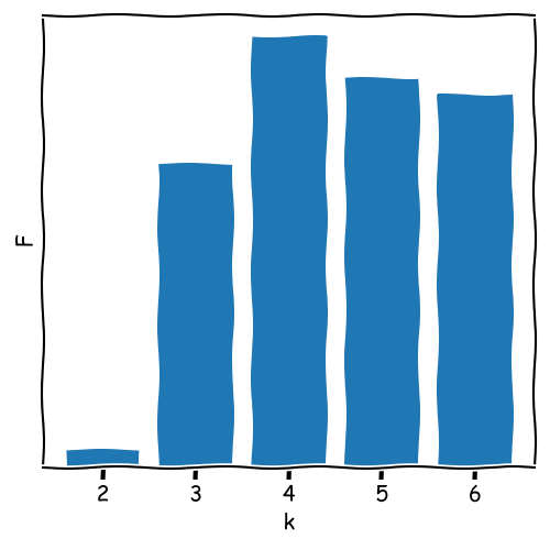
Evaluating the Clustering Results
To assess clustering quality, metrics such as the following are commonly used:
Inertia (within-cluster variance): Measures compactness within clusters; lower is better.
Silhouette Score: Measures cohesion and separation; ranges from -1 to 1.
ANOVA: Evaluates the separation between clusters by comparing between-cluster and within-cluster variance.
\[ \text{Inertia} = \sum_{i=1}^{k} \sum_{x \in C_i} \| x - \mu_i \|^2 \]
where \( x \) represents a data point in cluster \( C_i \), and \( \mu_i \) is the centroid of cluster \( C_i \).
\[ \text{Silhouette Score} = \frac{b - a}{\max(a, b)} \]
where \( a \) is the mean intra-cluster distance for each sample, and \( b \) is the mean nearest-cluster distance for each sample.
\[ F = \frac{\text{Between-Cluster Variance}}{\text{Within-Cluster Variance}} \]
Used in ANOVA to assess the ratio of variance between clusters to the variance within clusters.
Advantages and Limitations of K-Means
Advantages
Simple and efficient for large datasets with low computational complexity, especially when clusters are well-separated.
Can be easily adapted for different use cases, such as image compression and document clustering.
Works well with spherical-shaped clusters where data points are evenly distributed around a centroid.
Limitations
Requires the number of clusters, k, to be specified in advance, which can be challenging to
determine.
Sensitive to initial centroid placement, potentially leading to different clustering results in each run.
Not suitable for non-spherical clusters or clusters with varying sizes and densities.
Struggles with outliers, which can significantly impact the cluster centroids and overall result.
What is Principal Component Analysis (PCA)?
Principal Component Analysis (PCA) is a dimensionality reduction technique often
used in data science
and machine learning to simplify datasets by reducing the number of variables while preserving essential
information.
PCA works by identifying directions (principal components) along which the data varies the
most.
Applications include data visualization, noise reduction, and
feature extraction for machine learning.
Dimensionality Reduction through Axis Transformation
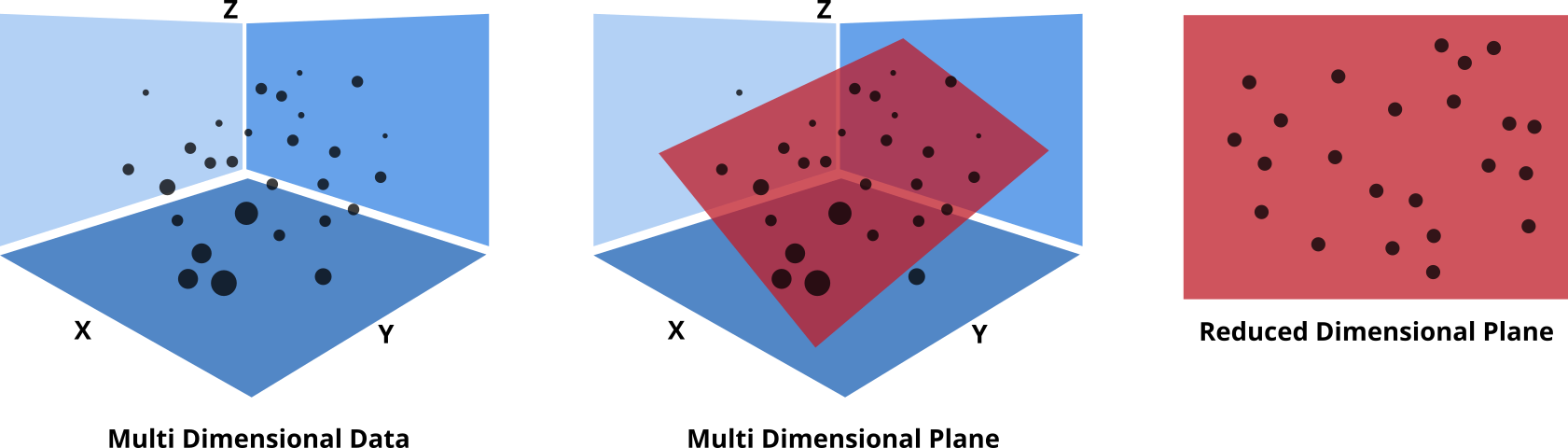
Coordinate Axes as a Matrix
The coordinate axes of a space can be represented as a matrix. In its simplest form, this is
the identity matrix, where all axes are perpendicular.
The identity matrix (or unity matrix) has values of 1 along its diagonal and 0 elsewhere,
representing standard perpendicular axes.
By modifying the angles between the axes, we can adjust this matrix to define
new coordinate systems.
                         Identity Matrix:
                         ┌     ┐
                         │ 1 0 │
                         │ 0 1 │
                         └     ┘
Example: Adjusting the identity matrix by changing angles between axes allows transformations to define new directions or rotations in data.
                       Identity Matrix:
                       ┌     ┐          ┌     ┐
                       │ 1 0 │  Strech  │ 2 0 │
                       │ 0 1 │  along   │ 0 1 │
                       └     ┘  x-axis  └     ┘
          coordinates:  (5, 3)    ->  s (10, 3)
Remember: Matrix x Vector means row-wise multiplication of the matrix with the vector. E.g.
2 * 5 + 0 * 3 and 0 * 5 + 1 * 3 in the example above.
Dimensionality Reduction through Axis Transformation
PCA reduces dimensions by transforming coordinate axes. It finds new axes,
principal components, where data varies most.
This is a mathematical axis transformation, projecting original data onto principal component
axes.
Example: With two features, x1 and x2, PCA rotates the axes to find
PC1 (highest variance), possibly discarding PC2 for dimensional reduction.
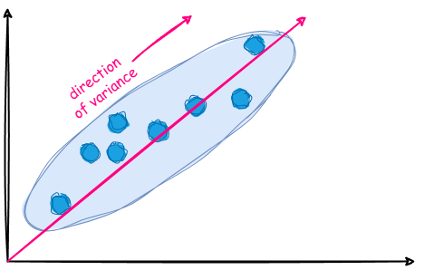
Covariance Matrix and Data Variance
The covariance matrix reveals directions in the data with maximum variation, guiding PCA to
choose the best transformation.
Each matrix element represents covariance between two features. Diagonal elements show
variance within each feature, while off-diagonal elements show relationships between features.
Formula for covariance between features \( x \) and \( y \):
\[
\text{cov}(x, y) = \frac{1}{n - 1} \sum_{i=1}^{n} (x_i - \bar{x})(y_i - \bar{y})
\]
Example of a 4x4 covariance matrix \( \Sigma \): \[ \begin{bmatrix} \text{var}(x_1) & \text{cov}(x_1, x_2) & \text{cov}(x_1, x_3) & \text{cov}(x_1, x_4) \\ \text{cov}(x_2, x_1) & \text{var}(x_2) & \text{cov}(x_2, x_3) & \text{cov}(x_2, x_4) \\ \text{cov}(x_3, x_1) & \text{cov}(x_3, x_2) & \text{var}(x_3) & \text{cov}(x_3, x_4) \\ \text{cov}(x_4, x_1) & \text{cov}(x_4, x_2) & \text{cov}(x_4, x_3) & \text{var}(x_4) \end{bmatrix} \]
Foundation of PCA Transformation: Eigenvectors and Eigenvalues
The covariance matrix shows how dimensions of the data correlate and spread. Each value
describes the joint variance between two dimensions.
The eigenvectors of the covariance matrix represent directions of the greatest variance in
the data. These define the new axes, known as principal components.
By projecting data onto the eigenvectors, we highlight the
primary directions of variation, reducing correlation between dimensions.
Retaining the largest eigenvalues reduces dimensionality, focusing on the primary sources of
information in the data.
Example: Covariance Matrix of a 4-Dimensional Dataset
Suppose we have a dataset with four features: x1, x2, x3, and
x4.
The covariance matrix reveals relationships between these features:
                         ┌                    ┐
                         │ 2.5  0.8  0.6  1.2 │
                   Cov = │ 0.8  1.9  0.4  0.9 │
                         │ 0.6  0.4  2.3  1.1 │
                         │ 1.2  0.9  1.1  3.2 │
                         └                    ┘
Diagonal elements (e.g., 2.5 for x1) show variance for each feature.
Off-diagonal values indicate covariance between features (e.g., 0.8 between
x1 and x2).
Features with high covariance are more similar. For example, x3 and x4 have
covariance 1.1, suggesting they vary similarly.
Low covariance between features like x1 and x3 means PCA will place less weight
on
this direction, focusing on features with higher covariance to capture more variance.
The eigenvectors of this matrix, aligned with principal components, will orient along directions with the highest variance, maximizing data spread along these axes.
Understanding Eigenvectors
An eigenvector of a matrix is a special vector that, when multiplied by the matrix,
changes only in scale, not direction.
For a matrix A and an eigenvector v, we have:
\[ A \cdot v = \lambda \cdot v \]
where λ is the eigenvalue that scales v.
In PCA, eigenvectors of the covariance matrix give directions for the principal components,
with the eigenvalues showing their importance (variance captured).
Example: For a 4D dataset, the eigenvectors might show directions of maximum spread,
while eigenvalues indicate the strength of each direction.
Example 2: original vec & transformed vec
                           ┌      ┐
                           │ 3  2 │
                       A = │ 1  5 │
                           └      ┘
1
Covariance Matrix and Its Eigenvectors & Eigenvalues
The covariance matrix of the data:
                           ┌                    ┐
                           │ 2.5  0.8  0.6  1.2 │
                     Cov = │ 0.8  1.9  0.4  0.9 │
                           │ 0.6  0.4  2.3  1.1 │
                           │ 1.2  0.9  1.1  3.2 │
                           └                    ┘
Eigenvector matrix and corresponding eigenvalues:
                         ┌                               ┐
                         │  1.617  -0.777  -3.007  0.731 │
                     V = │ -3.288   0.115  -2.068  0.522 │
                         │ -0.776  -0.819   3.786  0.601 │
                         │    1       1       1      1   │
                         └                               ┘
                     λ_1 ≈ 1.3, λ_2 ≈ 1.5, λ_3 ≈ 1.9, λ_4 ≈ 5.2
Each eigenvalue λ indicates the variance captured along the direction of its
eigenvector.
The eigenvectors v_4 and v_3 with the highest eigenvalues capture the most
variance and are the first and second principal components.
Interpreting the Role of Eigenvectors and Eigenvalues in PCA
Eigenvectors represent the new axes in PCA, also known as
principal components.
The individual values within an eigenvector describe how much each original feature
contributes to the principal component.
A larger value indicates that a specific feature plays a more significant role in this component.
Eigenvalues reflect the amount of variance captured by each principal component.
The sum of all eigenvalues represents the total variance in the data.
Higher eigenvalues mean a component captures more variance, ideally with the first few components covering a substantial portion.
If eigenvalues are distributed evenly, PCA might not significantly reduce dimensions, suggesting it may be less effective for the data.
Transforming Data: Loadings and Scores
To transform the data, we use the eigenvectors of the covariance matrix. These eigenvectors
form a new basis for the data.
Each data point is projected onto this new basis, creating two key components:
Scores: Represent the data points in the new coordinate system defined by the principal
components.
Loadings: Show how the original variables contribute to each principal component.
Transformation process:
                      Data × Eigenvectors = Scores
                      ┌       ┐   ┌                  ┐   ┌        ┐
                      │ x1 x2 │ × │ v_1   v_2  ...   │ = │  PC1   │
                      │ ...   │   │ ...   ...  ...   │   │  PC2   │
                      │ xN xN │   │ v_m   v_n  ...   │   │  ...   │
                      └       ┘   └                  ┘   └        ┘
Each row of Scores represents a transformed data point, and each column of
Loadings shows the contribution of each variable to a principal component.
PCA is data decomposition, breaking down the data into loadings \(l\) & scores \(s\). \[ Data = s \cdot l^T \] Where \(l^T\) is the transpose of the loadings matrix (loadings are the eigenvectors).
Working Example: PCA on Fruits Dataset
Different Fruits as Samples.
Apple, Banana, Lime, Grape, Pineapple
Different measurements methods as Features.
Sweetness, Weight, Price
Sourness, Color(Red), Color(Blue), Color(Green)
Sweetness Weight Price Sourness Color(R) Color(G) Color(B)
   9.0     995.6  5.0    1.0      246      255      38
   7.3     156.1  2.9    3.9      249       16      12
   5.3     143.6  2.1    3.4      250        9      28
   5.8     122.5  0.6    2.3      248      250       7
   6.9      99.8  1.3    1.9      251      255       9
   3.0      39.3  2.2    8.5        5      253       4
   5.4     158.4  3.2    3.3      255        7      11
   4.3     126.2  1.4    3.0      255      255       3
   3.4      58.6  1.7    7.0       15      254      15
   6.6     124.6  1.3    1.1      255      243      11
   7.8       7.7  4.6    3.8      115       12      99
   9.8     995.7  5.6    3.1      255      255      37
   8.5      18.1  4.5    2.2      137        9     127
   2.2      55.2  3.0    7.7        7      255       1
   7.8      13.3  4.7    2.7      140       13     123
   3.7      41.3  2.8    8.8        9      239       1
   2.2      44.4  1.9    8.0        8      255      18
   8.0    1000.8  5.0    1.5      255      255      48
   6.2     151.1  3.7    4.8      255       12       2
   7.3     129.2  1.2    0.0      248      233       5
   8.7     141.5  2.9    3.6      253        9       3
   7.2     122.8  1.4    2.9      255      249       7
   8.8    1005.9  6.4    0.4      253      255      58
   4.0      38.3  2.9    7.7       11      255       7
   7.7    1009.1  4.9    1.6      255      255      36
   8.1     984.8  5.3    1.1      253      255      33
   7.7      13.1  3.8    2.8      124        8     115
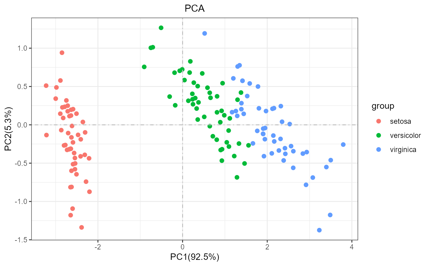
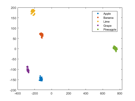
Working Example: PCA on Fruits Dataset < Scores Plot>
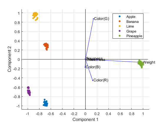
Working Example: PCA on Fruits Dataset < Bi-Plot>
Working Example: PCA on Fruits Dataset < Interpretation>
The PCA bi-plot shows the relationship between samples and features in the transformed space.
Samples are represented by points, while features are shown as vectors.
The length and direction of feature vectors indicate their importance and relationship to samples.
In this example, the first principal component (PC1) is strongly influenced weight, while the second principal component (PC2) is driven by color features.
Advantages and Limitations of PCA
Advantages of PCA
Dimensionality Reduction: Simplifies datasets by reducing variables, preserving core
information.
Noise Reduction: Filters noise by focusing on components with the highest variance.
Improved Visualization: Enables visualization of high-dimensional data in 2D or 3D.
Feature Extraction: Highlights uncorrelated variables, making dominant features clear.
Limitations of PCA
Linear Assumptions: Captures linear relationships but may miss non-linear structures.
Loss of Interpretability: Principal components lack intuitive meaning compared to original
features.
Variance-Based Selection: Ignores low-variance components that may still hold relevant
information.
Scaling Sensitivity: Results can vary with inconsistent feature scaling.
Excursion to Linear Discriminant Analysis (LDA)
Linear Discriminant Analysis (LDA) is similar to PCA, but with a focus on distinguishing
between predefined groups.
Instead of maximizing overall variance, LDA aims to maximize separation between
groups.
LDA uses the within-group covariance matrix inverse, multiplied by the
between-group covariance matrix, to find new axes.
\[ C = \Sigma_w^{-1} \cdot \Sigma_b \]
The new axes (or discriminant components) in LDA are chosen to best separate the groups, not
just capture variance.
Applications: Often used in classification tasks, as it enhances differences between
categories, improving separability.
Limitations: LDA assumes normally distributed data within each group and may struggle with
non-linear boundaries.
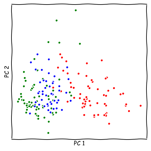
LDA vs. PCA
Seminar Material
We will have a look on a dataset of 178 different Wines.
Multiple measurements were taken for each wine.
Using PCA, we will try to reduce the dimensionality of the dataset.
Using K-Means, we will try to cluster the wines into different groups.
Download the data set here: Wine.csv